The Trump budget doesn’t spare seniors
President Trump’s proposed 2021 budget claims to help the “most vulnerable populations,” including seniors. But vulnerable older Americans are among those who would be most hurt if this draconian budget were ever enacted.
The budget would slash Medicaid and non-defense discretionary spending, eliminating or drastically shrinking programs targeted at low-income people, including programs benefiting seniors, such as the Low Income Home Energy Assistance Program. At first glance, the administration appears to spare middle-class seniors, a group with high voter turnout that tends to support the president and his party. Despite the president’s hints that Social Security and Medicare will be on the chopping block after the election, the budget would spare retirement benefits (except those for federal employees) and claims to achieve Medicare savings only by eliminating “excessive spending and distortionary payment incentives” while “preserv[ing] benefits and access to care.”
Some Medicare provisions in the president’s budget, such as site-neutral payments across different types of facilities, address genuine problems in how Medicare is administered. But the nearly half trillion in proposed savings from Medicare over 10 years includes provisions that would indirectly affect Medicare beneficiaries’ access to care, such as reducing payments to partially cover unpaid medical bills for Medicare beneficiaries. Since unlimited out-of-pocket expenses are a major cause of bankruptcy for older Americans in poor health, reducing these reimbursements would cause some providers to avoid treating Medicare patients who have expensive conditions and limited resources—and would surely lead to hospital and clinic closures in underserved areas. Middle-class seniors and providers who treat them wouldn’t be spared, since lower-middle-class seniors ineligible for Medicaid are those most likely to spend a high share of their income on health care. The problem of uncompensated care would be compounded by the administration’s attempts to roll back Medicaid expansion under the Affordable Care Act (ACA), which has helped hospitals treating low-income and uninsured patients in expansion states.
Top five Valentine’s Day gifts ideas for U.S. workers: Nothing spells ‘romance’ like a fair wage and quality jobs
That’s why we decided to sum up what we think are the top five Valentine’s Day gifts ideas for working people across the country.
Power through collective action!
Our economy is out of balance. Corporations and CEOs hold too much power and wealth, and working people know it. Workers are mobilizing, organizing, protesting, and striking at a level not seen in decades, and they are winning pay raises and other real change by using their collective voices.
But, the fact is, it is still too difficult for working people to form a union at their workplace when they want to. The law gives employers too much power and puts too many roadblocks in the way of workers trying to organize a union. The Protecting the Right to Organize (PRO) Act will go a long way toward restoring workers’ right to join together to bargain for better wages and working conditions by streamlining the process when workers form a union, ensuring that they are successful in negotiating a first agreement, and holding employers accountable when they violate labor law. The U.S. Senate should join the House of Representatives and pass the PRO Act in order to restore power to working people.
Affording bread…and roses
The real (inflation-adjusted) minimum wage is now roughly 30 percent lower than it was in 1968, and it has been more than 10 years since congress raised the minimum wage—the longest stretch in history. To end this shameful streak, it is incumbent upon the Senate to take up and pass the Raise the Wage Act immediately. Raising the federal minimum wage to $15 by 2025 would lift wages for 33.5 million workers across the country—more than one-fifth of the wage-earning workforce. The increase would boost total annual wages for these low-wage workers by $92.5 billion, lifting annual earnings for the average affected year-round worker by $2,800. Recent survey data have shown that 74% of U.S. workers live paycheck to paycheck. Policymakers should give working people the ability to make ends meet—but also the ability to treat themselves occasionally.
Failure to raise the federal minimum wage has taken thousands of dollars out of the pockets of minimum wage workers: The real value of the minimum wage (adjusted for inflation) is 17% less than 10 years ago and 31% less than in 1968
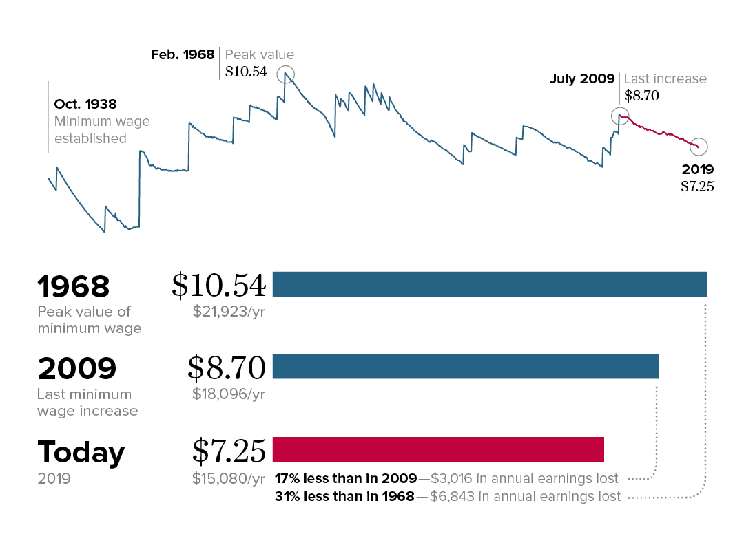

Note: All values are in June 2019 dollars, adjusted using the CPI-U-RS.
Source: Adapted from Figure C in David Cooper, Elise Gould, and Ben Zipperer, Low-Wage Workers Are Suffering from a Decline in the Real Value of the Federal Minimum Wage, Economic Policy Institute, August 2019).
Source: Adapted from Figure C in David Cooper, Elise Gould, and Ben Zipperer, Low-Wage Workers Are Suffering from a Decline in the Real Value of the Federal Minimum Wage, Economic Policy Institute, August 2019). The figure reflects EPI analysis of historical minimum wage data in the Fair Labor Standards Act and amendments.
Pay workers for their hours worked, or give them their time back
The U.S. Department of Labor announced in September its final overtime rule, which will set the salary threshold under which salaried workers are automatically entitled to overtime pay to $35,568 a year. The rule leaves behind millions of workers who would have received overtime protections under the much stronger rule, published in 2016, that Trump administration chose to abandon. A stronger overtime protection would pay more workers for working more than 40 hours a week, or allow them extra time with their families.
Seven states have already taken steps to raise the overtime threshold, but without further action, it’s estimated that 8.2 million workers who would have benefited from the 2016 rule will be left behind by the Trump administration’s rule, including 3.2 million workers who would have gotten new overtime protections under the 2016 rule and 5.0 million who would have gotten strengthened overtime protections under the 2016 rule. States should follow suit and extend the overtime protections so workers don’t continue to lose out on their hard-earned wages.
Let your workers move on
At least 36 million workers—27.8% of the private-sector workforce—are required to enter noncompete agreements. Noncompete agreements are employment provisions that ban workers at one company from going to work for, or starting, a competing business within a certain period of time after leaving a job. Establishments with high pay or high levels of education among workers are more likely to use noncompetes, but noncompetes agreements are also common in workplaces with low pay and low levels of education. More than a quarter (29.0%) of private-sector workers with an average hourly wage below $13.00 require noncompetes for all their workers. Noncompetes are part of a disturbing trend of employers requiring workers to sign away their rights. Noncompetes may be contributing to weak wage growth, given that changing jobs is how workers often get a raise. And given that noncompetes limit the ability of individuals to start businesses or take other jobs, it also is not difficult to see that noncompetes may be contributing to the declines in dynamism in the U.S. labor market. Congress should pass the bipartisan legislation, the Workforce Mobility Act of 2019, to prohibit noncompete agreements.

Labor protections for Uber drivers shuttling around Valentine’s couples
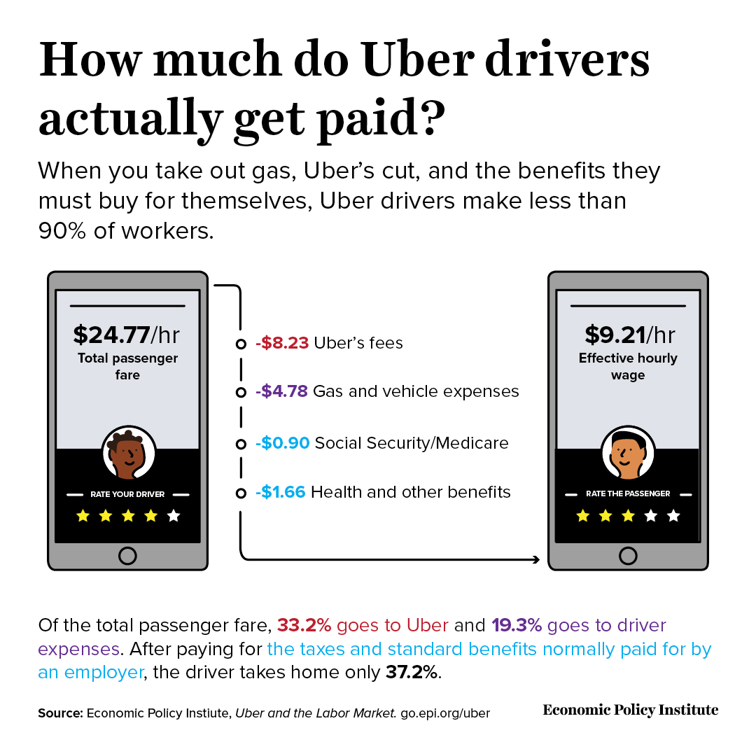
The General Counsel of the National Labor Relations Board recently released a memo claiming that Uber drivers are independent contractors, not employees of Uber. The reality is that these drivers have very little entrepreneurial freedom: Drivers can’t raise revenues because they can’t control prices or expand their customer base through marketing. Unlike a typical enterprise, Uber drivers do not build earnings as they get more experience. Uber drivers are not able to choose their customers—drivers are penalized for rejecting or not accepting trips. And after accounting for Uber’s commissions and fees and vehicle expenses, and taking into account the cost of a modest package of health insurance and other benefits equivalent to those earned by W-2 workers, Uber drivers earn the equivalent of $9.21 in hourly wages—less than what is earned by 90% of all other wage and salary earners, and below the minimum wage in 13 of the 20 major urban markets where Uber operates.
Recently, AB5 went into effect in California, a set of protections aimed at combatting the misclassification of workers as independent contractors, helping ensure that California’s employees have access to basic labor and employment protections denied to independent contractors including: minimum wage and overtime protections, paid sick days and family leave, workers’ compensation benefits, and unemployment insurance benefits. Policymakers across the country should take notice and provide similar protections to workers in their states.
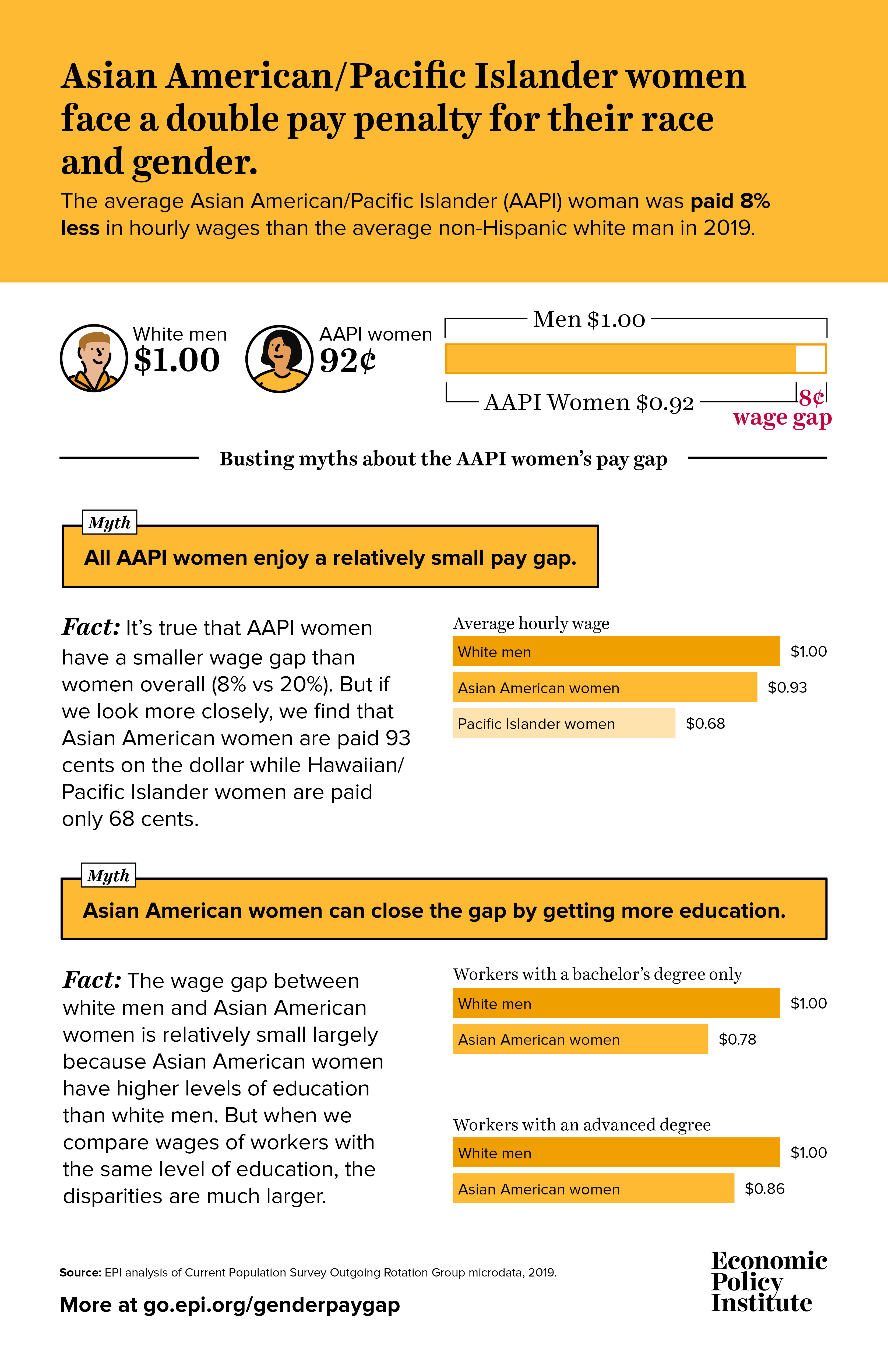
AAPI women face a double pay penalty for race and gender
Asian American/Pacific Islander (AAPI) Equal Pay Day is February 11. It marks the number of days into 2020 that AAPI women have to work to make the same amount as their white male counterparts were paid in 2019. Put another way, the average AAPI woman needs to work almost an extra month and a half to make up for the shortfall in annual earnings relative to the average non-Hispanic white man.
The infographic below takes a closer look at the data to debunk commonly held myths about the AAPI women’s pay gap. Specifically, all AAPI women do not face a relatively small pay gap—Asian American women are paid 93 cents on the dollar, while Hawaiian/Pacific Islander women are paid only 68 cents.
Further, Asian American women can’t just educate their way out of the pay gap. Asian American women have higher levels of education than white men, and when comparing wages of workers with the same level of education, the disparities are much larger. Asian American women with a bachelor’s degree only are paid 22% less than their white male counterparts and those with an advanced degree are paid 14% less.
Declining trade balances disguise continued growth in the non-oil trade deficit
The overall goods and services trade deficit declined 1.7% ($10.9 billion) in 2019, while the total deficit in goods trade fell 2.4% ($21.4 billion). However, the U.S. trade deficit in non-oil goods, which is dominated by trade in manufactured products, increased 1.8% in 2019. Aside from petroleum, trade was a net drag on the economy in 2019 and on manufacturing, in particular.
The small decline in overall U.S. trade deficits follows an 18.3% increase in the goods trade deficit in the first two years of the Trump administration. Taken altogether, the U.S. goods trade deficit increased $116.2 billion (15.5%) in the first three years of the Trump Administration. It has proven neither quick nor easy to reduce the growing U.S. goods trade deficit.
The petroleum products deficit decreased 72.6% in 2019, masking the 1.8% increase in the non-oil goods trade deficit within the overall 2.4% decline in the U.S. goods trade balance. The fracking revolution has resulted in a significant reduction in oil imports (13.9%) and a small increase in petroleum exports (2.8%).
Recent changes in petroleum trade yield this shocking factoid: The United States became a net exporter of petroleum products for the last four months of 2019. This reflects a key element of Trump’s trade “strategy” to export liquefied natural gas (LNG) to the rest of the world, which comes at a steep cost. This will drive up U.S. prices for natural gas and oil, despite the fact that low energy prices were a key element of the mini-recovery in US manufacturing exports. Increased LNG exports will hurt U.S. consumers by increasing fuel costs, heightening risks of transport and catastrophic port explosions, and exacerbating global warming and air pollution levels in the country as a whole.
What to watch on jobs day: Large downward revisions in employment expected
On Friday, the Bureau of Labor Statistics (BLS) will revise nonfarm payroll employment, hours, and earnings data to reflect the annual benchmark process in the establishment survey. Each year, the BLS benchmarks total nonfarm payroll employment to state unemployment insurance tax records. In August 2019, BLS released preliminary benchmark revisions to payroll employment for April 2018 through March 2019, but revisions don’t get officially incorporated into the historical numbers until the final revisions are released. While revisions in most years tend to be relatively small, this year’s preliminary revisions came in much higher. The preliminary estimate of the benchmark revision indicates a downward adjustment to March 2019 total nonfarm employment of -501,000. This means that between April 2018 and March of 2019, there were a half million fewer jobs created than initially reported. Over the last ten years, preliminary revisions averaged about -92,000, so -501,000 is very large in comparison. And, usually the difference between the preliminary revisions and the final revisions is plus or minus 40,000. Therefore, it’s likely tomorrow’s final revisions will also be around 500,000 fewer jobs in that period.
The revisions will also provide details on changes in the initial payroll employment estimates by sector. For instance, in the preliminary release, the revisions were located primarily in “leisure and hospitality”, “professional and business services”, and “retail trade” with downward revisions of -175,000, -163,000, and -146,400, respectively. On Friday, the historical data will reflect the final benchmarks overall and by sector.
Tracking trends in nominal wage growth
Turning to nominal wage growth, the most important economic indicator to watch in 2020, last month there was a large drop for production/nonsupervisory workers. The figure below charts year-over-year changes in private-sector nominal average hourly earnings for “all nonfarm employees” as well as “production/nonsupervisory workers.” After remaining consistently higher than “all nonfarm” for nearly a year and at or above 3.4% for much of that time, it fell to 3.0% in December, its lowest point since September 2018. This begs the question of whether this is simply a blip and production/nonsupervisory workers will continue to pull away or if the separation in growth rates between the two over the last year was mostly statistical noise.
At this point in the recovery—with unemployment at or below 4.0% for 22 months—wage growth remains lower than expected. As employment growth consistently remains higher than working-age population growth, more and more workers are pulled into the labor force and finding jobs. As this slack gets absorbed, workers should be getting scarcer and scarcer. Therefore, employers would typically have to pay more to attract and retain the workers they want. After increasing in 2018, wage growth for all nonfarm employees has slowed for much of 2019 and remains below target levels.
Nominal wage growth has been far below target in the recovery: Year-over-year change in private-sector nominal average hourly earnings, 2007–2019
| Date | All nonfarm employees | Production/nonsupervisory workers |
|---|---|---|
| Mar-2007 | 3.44% | 4.11% |
| Apr-2007 | 3.08% | 3.79% |
| May-2007 | 3.48% | 4.14% |
| Jun-2007 | 3.56% | 4.19% |
| Jul-2007 | 3.25% | 4.05% |
| Aug-2007 | 3.35% | 3.98% |
| Sep-2007 | 3.14% | 4.09% |
| Oct-2007 | 3.08% | 3.78% |
| Nov-2007 | 3.07% | 3.83% |
| Dec-2007 | 2.97% | 3.81% |
| Jan-2008 | 2.91% | 3.80% |
| Feb-2008 | 2.80% | 3.79% |
| Mar-2008 | 3.04% | 3.83% |
| Apr-2008 | 2.84% | 3.76% |
| May-2008 | 3.07% | 3.69% |
| Jun-2008 | 2.77% | 3.56% |
| Jul-2008 | 3.05% | 3.67% |
| Aug-2008 | 3.33% | 3.89% |
| Sep-2008 | 3.23% | 3.64% |
| Oct-2008 | 3.27% | 3.81% |
| Nov-2008 | 3.60% | 3.91% |
| Dec-2008 | 3.59% | 3.90% |
| Jan-2009 | 3.63% | 3.72% |
| Feb-2009 | 3.43% | 3.65% |
| Mar-2009 | 3.28% | 3.47% |
| Apr-2009 | 3.42% | 3.35% |
| May-2009 | 2.93% | 3.06% |
| Jun-2009 | 2.83% | 2.88% |
| Jul-2009 | 2.69% | 2.71% |
| Aug-2009 | 2.44% | 2.70% |
| Sep-2009 | 2.44% | 2.75% |
| Oct-2009 | 2.53% | 2.68% |
| Nov-2009 | 2.19% | 2.67% |
| Dec-2009 | 1.91% | 2.50% |
| Jan-2010 | 2.05% | 2.66% |
| Feb-2010 | 2.09% | 2.55% |
| Mar-2010 | 1.81% | 2.27% |
| Apr-2010 | 1.76% | 2.38% |
| May-2010 | 1.90% | 2.59% |
| Jun-2010 | 1.76% | 2.53% |
| Jul-2010 | 1.85% | 2.42% |
| Aug-2010 | 1.75% | 2.36% |
| Sep-2010 | 1.84% | 2.19% |
| Oct-2010 | 1.93% | 2.45% |
| Nov-2010 | 1.65% | 2.13% |
| Dec-2010 | 1.79% | 2.02% |
| Jan-2011 | 1.92% | 2.28% |
| Feb-2011 | 1.87% | 2.06% |
| Mar-2011 | 1.87% | 2.06% |
| Apr-2011 | 1.91% | 2.16% |
| May-2011 | 2.04% | 2.10% |
| Jun-2011 | 2.13% | 2.05% |
| Jul-2011 | 2.30% | 2.26% |
| Aug-2011 | 1.99% | 1.94% |
| Sep-2011 | 1.94% | 1.99% |
| Oct-2011 | 2.07% | 1.88% |
| Nov-2011 | 2.02% | 1.82% |
| Dec-2011 | 1.98% | 1.77% |
| Jan-2012 | 1.71% | 1.35% |
| Feb-2012 | 1.79% | 1.45% |
| Mar-2012 | 2.10% | 1.76% |
| Apr-2012 | 2.09% | 1.65% |
| May-2012 | 1.78% | 1.39% |
| Jun-2012 | 2.00% | 1.54% |
| Jul-2012 | 1.77% | 1.44% |
| Aug-2012 | 1.86% | 1.33% |
| Sep-2012 | 2.03% | 1.54% |
| Oct-2012 | 1.51% | 1.18% |
| Nov-2012 | 1.90% | 1.43% |
| Dec-2012 | 2.24% | 1.69% |
| Jan-2013 | 2.24% | 1.84% |
| Feb-2013 | 2.15% | 2.04% |
| Mar-2013 | 1.93% | 1.88% |
| Apr-2013 | 2.05% | 1.83% |
| May-2013 | 2.14% | 1.93% |
| Jun-2013 | 2.13% | 2.03% |
| Jul-2013 | 2.00% | 1.97% |
| Aug-2013 | 2.26% | 2.23% |
| Sep-2013 | 2.04% | 2.22% |
| Oct-2013 | 2.25% | 2.32% |
| Nov-2013 | 2.24% | 2.37% |
| Dec-2013 | 1.85% | 2.21% |
| Jan-2014 | 1.89% | 2.31% |
| Feb-2014 | 2.27% | 2.55% |
| Mar-2014 | 2.10% | 2.30% |
| Apr-2014 | 1.93% | 2.29% |
| May-2014 | 2.09% | 2.44% |
| Jun-2014 | 1.96% | 2.24% |
| Jul-2014 | 2.04% | 2.33% |
| Aug-2014 | 2.16% | 2.43% |
| Sep-2014 | 2.08% | 2.22% |
| Oct-2014 | 2.03% | 2.27% |
| Nov-2014 | 2.03% | 2.22% |
| Dec-2014 | 1.99% | 1.92% |
| Jan-2015 | 2.19% | 2.01% |
| Feb-2015 | 1.93% | 1.66% |
| Mar-2015 | 2.22% | 1.95% |
| Apr-2015 | 2.26% | 2.00% |
| May-2015 | 2.34% | 2.14% |
| Jun-2015 | 2.25% | 2.14% |
| Jul-2015 | 2.17% | 2.04% |
| Aug-2015 | 2.20% | 1.98% |
| Sep-2015 | 2.28% | 2.08% |
| Oct-2015 | 2.52% | 2.37% |
| Nov-2015 | 2.43% | 2.12% |
| Dec-2015 | 2.47% | 2.51% |
| Jan-2016 | 2.55% | 2.40% |
| Feb-2016 | 2.42% | 2.50% |
| Mar-2016 | 2.45% | 2.49% |
| Apr-2016 | 2.61% | 2.58% |
| May-2016 | 2.40% | 2.33% |
| Jun-2016 | 2.60% | 2.48% |
| Jul-2016 | 2.76% | 2.62% |
| Aug-2016 | 2.55% | 2.51% |
| Sep-2016 | 2.63% | 2.46% |
| Oct-2016 | 2.66% | 2.41% |
| Nov-2016 | 2.61% | 2.50% |
| Dec-2016 | 2.65% | 2.50% |
| Jan-2017 | 2.40% | 2.39% |
| Feb-2017 | 2.72% | 2.34% |
| Mar-2017 | 2.55% | 2.29% |
| Apr-2017 | 2.47% | 2.24% |
| May-2017 | 2.54% | 2.33% |
| Jun-2017 | 2.50% | 2.32% |
| Jul-2017 | 2.57% | 2.32% |
| Aug-2017 | 2.57% | 2.31% |
| Sep-2017 | 2.83% | 2.59% |
| Oct-2017 | 2.32% | 2.16% |
| Nov-2017 | 2.47% | 2.35% |
| Dec-2017 | 2.74% | 2.48% |
| Jan-2018 | 2.81% | 2.47% |
| Feb-2018 | 2.57% | 2.47% |
| Mar-2018 | 2.80% | 2.74% |
| Apr-2018 | 2.79% | 2.78% |
| May-2018 | 2.94% | 2.91% |
| Jun-2018 | 2.93% | 2.91% |
| Jul-2018 | 2.85% | 2.85% |
| Aug-2018 | 3.18% | 3.12% |
| Sep-2018 | 2.98% | 3.02% |
| Oct-2018 | 3.32% | 3.25% |
| Nov-2018 | 3.31% | 3.37% |
| Dec-2018 | 3.34% | 3.50% |
| Jan-2019 | 3.18% | 3.35% |
| Feb-2019 | 3.40% | 3.44% |
| Mar-2019 | 3.24% | 3.38% |
| Apr-2019 | 3.16% | 3.33% |
| May-2019 | 3.08% | 3.36% |
| Jun-2019 | 3.18% | 3.35% |
| Jul-2019 | 3.25% | 3.52% |
| Aug-2019 | 3.23% | 3.51% |
| Sep-2019 | 3.00% | 3.54% |
| Oct-2019 | 3.11% | 3.62% |
| Nov-2019 | 3.14% | 3.39% |
| Dec-2019 | 2.87% | 3.03% |
* Nominal wage growth consistent with the Federal Reserve Board’s 2 percent inflation target, 1.5 percent productivity growth, and a stable labor share of income
Source: EPI analysis of Bureau of Labor Statistics Current Employment Statistics public data series
On Friday, the BLS will also be employing new population controls in the Current Population Survey (CPS) starting in January 2020. Unlike the establishment survey, these changes to the CPS are not updated historically so caution should be exercised when making comparisons with data for December 2019 or earlier periods. The BLS is also making some changes to their methodology in terms of providing new seasonally adjusted series for measures of labor market underutilization as well as beginning to include both those in opposite-sex and same-sex marriages in estimates of married persons.
The new benchmarks to the establishment survey as well as revisions to the household survey will provide much fodder for thought on Friday morning. And, wage growth continues to be the most important indicator to watch as it lags behind overall improvements in the labor market.
Trump’s ‘blue-collar boom’ is likely a dud
In his State of the Union address tonight, President Trump plans to extol the “blue-collar boom” in the economy along with his purported “great American comeback.” He’ll claim this based on two recent signature trade deals—the United States-Mexico-Canada Agreement (USMCA) and a “phase one” deal with China. Unfortunately, both agreements will likely to lead to more outsourcing and job loss for U.S. workers, and the facts just don’t support Trump’s claims about the broader economy.
Trump comes from a world that has ardently championed globalization, like many of his predecessors. However, that approach has decimated U.S. manufacturing over the past 20 years, eliminating nearly 5 million good factory jobs as shown in Figure A, below. Nearly 90,000 U.S. factories have been lost as well.
U.S. manufacturing employment, January 1970–December 2019 (millions of jobs)
| Date | Manufacturing employment (millions of jobs) |
|---|---|
| 1970-01-01 | 18.424 |
| 1970-02-01 | 18.361 |
| 1970-03-01 | 18.36 |
| 1970-04-01 | 18.207 |
| 1970-05-01 | 18.029 |
| 1970-06-01 | 17.93 |
| 1970-07-01 | 17.877 |
| 1970-08-01 | 17.779 |
| 1970-09-01 | 17.692 |
| 1970-10-01 | 17.173 |
| 1970-11-01 | 17.024 |
| 1970-12-01 | 17.309 |
| 1971-01-01 | 17.28 |
| 1971-02-01 | 17.216 |
| 1971-03-01 | 17.154 |
| 1971-04-01 | 17.149 |
| 1971-05-01 | 17.225 |
| 1971-06-01 | 17.139 |
| 1971-07-01 | 17.126 |
| 1971-08-01 | 17.115 |
| 1971-09-01 | 17.154 |
| 1971-10-01 | 17.126 |
| 1971-11-01 | 17.166 |
| 1971-12-01 | 17.202 |
| 1972-01-01 | 17.283 |
| 1972-02-01 | 17.361 |
| 1972-03-01 | 17.447 |
| 1972-04-01 | 17.508 |
| 1972-05-01 | 17.602 |
| 1972-06-01 | 17.641 |
| 1972-07-01 | 17.556 |
| 1972-08-01 | 17.741 |
| 1972-09-01 | 17.774 |
| 1972-10-01 | 17.893 |
| 1972-11-01 | 18.005 |
| 1972-12-01 | 18.158 |
| 1973-01-01 | 18.276 |
| 1973-02-01 | 18.41 |
| 1973-03-01 | 18.493 |
| 1973-04-01 | 18.53 |
| 1973-05-01 | 18.564 |
| 1973-06-01 | 18.606 |
| 1973-07-01 | 18.598 |
| 1973-08-01 | 18.629 |
| 1973-09-01 | 18.609 |
| 1973-10-01 | 18.702 |
| 1973-11-01 | 18.773 |
| 1973-12-01 | 18.82 |
| 1974-01-01 | 18.788 |
| 1974-02-01 | 18.727 |
| 1974-03-01 | 18.7 |
| 1974-04-01 | 18.702 |
| 1974-05-01 | 18.688 |
| 1974-06-01 | 18.69 |
| 1974-07-01 | 18.656 |
| 1974-08-01 | 18.57 |
| 1974-09-01 | 18.492 |
| 1974-10-01 | 18.364 |
| 1974-11-01 | 18.077 |
| 1974-12-01 | 17.693 |
| 1975-01-01 | 17.344 |
| 1975-02-01 | 17.004 |
| 1975-03-01 | 16.853 |
| 1975-04-01 | 16.759 |
| 1975-05-01 | 16.746 |
| 1975-06-01 | 16.69 |
| 1975-07-01 | 16.678 |
| 1975-08-01 | 16.824 |
| 1975-09-01 | 16.904 |
| 1975-10-01 | 16.984 |
| 1975-11-01 | 17.025 |
| 1975-12-01 | 17.14 |
| 1976-01-01 | 17.287 |
| 1976-02-01 | 17.384 |
| 1976-03-01 | 17.47 |
| 1976-04-01 | 17.541 |
| 1976-05-01 | 17.513 |
| 1976-06-01 | 17.521 |
| 1976-07-01 | 17.524 |
| 1976-08-01 | 17.596 |
| 1976-09-01 | 17.665 |
| 1976-10-01 | 17.548 |
| 1976-11-01 | 17.682 |
| 1976-12-01 | 17.719 |
| 1977-01-01 | 17.803 |
| 1977-02-01 | 17.843 |
| 1977-03-01 | 17.941 |
| 1977-04-01 | 18.024 |
| 1977-05-01 | 18.107 |
| 1977-06-01 | 18.192 |
| 1977-07-01 | 18.259 |
| 1977-08-01 | 18.276 |
| 1977-09-01 | 18.334 |
| 1977-10-01 | 18.356 |
| 1977-11-01 | 18.419 |
| 1977-12-01 | 18.531 |
| 1978-01-01 | 18.593 |
| 1978-02-01 | 18.639 |
| 1978-03-01 | 18.699 |
| 1978-04-01 | 18.772 |
| 1978-05-01 | 18.848 |
| 1978-06-01 | 18.919 |
| 1978-07-01 | 18.951 |
| 1978-08-01 | 19.006 |
| 1978-09-01 | 19.068 |
| 1978-10-01 | 19.142 |
| 1978-11-01 | 19.257 |
| 1978-12-01 | 19.334 |
| 1979-01-01 | 19.388 |
| 1979-02-01 | 19.409 |
| 1979-03-01 | 19.453 |
| 1979-04-01 | 19.45 |
| 1979-05-01 | 19.509 |
| 1979-06-01 | 19.553 |
| 1979-07-01 | 19.531 |
| 1979-08-01 | 19.406 |
| 1979-09-01 | 19.442 |
| 1979-10-01 | 19.39 |
| 1979-11-01 | 19.299 |
| 1979-12-01 | 19.301 |
| 1980-01-01 | 19.282 |
| 1980-02-01 | 19.219 |
| 1980-03-01 | 19.217 |
| 1980-04-01 | 18.973 |
| 1980-05-01 | 18.726 |
| 1980-06-01 | 18.49 |
| 1980-07-01 | 18.276 |
| 1980-08-01 | 18.414 |
| 1980-09-01 | 18.445 |
| 1980-10-01 | 18.506 |
| 1980-11-01 | 18.601 |
| 1980-12-01 | 18.64 |
| 1981-01-01 | 18.639 |
| 1981-02-01 | 18.613 |
| 1981-03-01 | 18.647 |
| 1981-04-01 | 18.711 |
| 1981-05-01 | 18.766 |
| 1981-06-01 | 18.789 |
| 1981-07-01 | 18.785 |
| 1981-08-01 | 18.748 |
| 1981-09-01 | 18.712 |
| 1981-10-01 | 18.566 |
| 1981-11-01 | 18.409 |
| 1981-12-01 | 18.223 |
| 1982-01-01 | 18.047 |
| 1982-02-01 | 17.981 |
| 1982-03-01 | 17.857 |
| 1982-04-01 | 17.683 |
| 1982-05-01 | 17.588 |
| 1982-06-01 | 17.43 |
| 1982-07-01 | 17.278 |
| 1982-08-01 | 17.16 |
| 1982-09-01 | 17.074 |
| 1982-10-01 | 16.853 |
| 1982-11-01 | 16.722 |
| 1982-12-01 | 16.69 |
| 1983-01-01 | 16.705 |
| 1983-02-01 | 16.706 |
| 1983-03-01 | 16.711 |
| 1983-04-01 | 16.794 |
| 1983-05-01 | 16.885 |
| 1983-06-01 | 16.96 |
| 1983-07-01 | 17.059 |
| 1983-08-01 | 17.118 |
| 1983-09-01 | 17.255 |
| 1983-10-01 | 17.367 |
| 1983-11-01 | 17.479 |
| 1983-12-01 | 17.551 |
| 1984-01-01 | 17.63 |
| 1984-02-01 | 17.728 |
| 1984-03-01 | 17.806 |
| 1984-04-01 | 17.872 |
| 1984-05-01 | 17.916 |
| 1984-06-01 | 17.967 |
| 1984-07-01 | 18.013 |
| 1984-08-01 | 18.034 |
| 1984-09-01 | 18.019 |
| 1984-10-01 | 18.024 |
| 1984-11-01 | 18.016 |
| 1984-12-01 | 18.023 |
| 1985-01-01 | 18.009 |
| 1985-02-01 | 17.966 |
| 1985-03-01 | 17.939 |
| 1985-04-01 | 17.886 |
| 1985-05-01 | 17.855 |
| 1985-06-01 | 17.819 |
| 1985-07-01 | 17.776 |
| 1985-08-01 | 17.756 |
| 1985-09-01 | 17.718 |
| 1985-10-01 | 17.708 |
| 1985-11-01 | 17.697 |
| 1985-12-01 | 17.693 |
| 1986-01-01 | 17.686 |
| 1986-02-01 | 17.663 |
| 1986-03-01 | 17.624 |
| 1986-04-01 | 17.616 |
| 1986-05-01 | 17.593 |
| 1986-06-01 | 17.53 |
| 1986-07-01 | 17.497 |
| 1986-08-01 | 17.489 |
| 1986-09-01 | 17.498 |
| 1986-10-01 | 17.477 |
| 1986-11-01 | 17.472 |
| 1986-12-01 | 17.478 |
| 1987-01-01 | 17.465 |
| 1987-02-01 | 17.499 |
| 1987-03-01 | 17.507 |
| 1987-04-01 | 17.525 |
| 1987-05-01 | 17.542 |
| 1987-06-01 | 17.537 |
| 1987-07-01 | 17.593 |
| 1987-08-01 | 17.63 |
| 1987-09-01 | 17.691 |
| 1987-10-01 | 17.729 |
| 1987-11-01 | 17.775 |
| 1987-12-01 | 17.809 |
| 1988-01-01 | 17.79 |
| 1988-02-01 | 17.823 |
| 1988-03-01 | 17.844 |
| 1988-04-01 | 17.874 |
| 1988-05-01 | 17.892 |
| 1988-06-01 | 17.916 |
| 1988-07-01 | 17.926 |
| 1988-08-01 | 17.891 |
| 1988-09-01 | 17.914 |
| 1988-10-01 | 17.966 |
| 1988-11-01 | 18.003 |
| 1988-12-01 | 18.025 |
| 1989-01-01 | 18.057 |
| 1989-02-01 | 18.055 |
| 1989-03-01 | 18.06 |
| 1989-04-01 | 18.055 |
| 1989-05-01 | 18.04 |
| 1989-06-01 | 18.013 |
| 1989-07-01 | 17.98 |
| 1989-08-01 | 17.964 |
| 1989-09-01 | 17.922 |
| 1989-10-01 | 17.895 |
| 1989-11-01 | 17.886 |
| 1989-12-01 | 17.881 |
| 1990-01-01 | 17.797 |
| 1990-02-01 | 17.893 |
| 1990-03-01 | 17.868 |
| 1990-04-01 | 17.845 |
| 1990-05-01 | 17.797 |
| 1990-06-01 | 17.776 |
| 1990-07-01 | 17.704 |
| 1990-08-01 | 17.649 |
| 1990-09-01 | 17.609 |
| 1990-10-01 | 17.577 |
| 1990-11-01 | 17.428 |
| 1990-12-01 | 17.395 |
| 1991-01-01 | 17.33 |
| 1991-02-01 | 17.211 |
| 1991-03-01 | 17.14 |
| 1991-04-01 | 17.093 |
| 1991-05-01 | 17.07 |
| 1991-06-01 | 17.044 |
| 1991-07-01 | 17.015 |
| 1991-08-01 | 17.025 |
| 1991-09-01 | 17.01 |
| 1991-10-01 | 16.999 |
| 1991-11-01 | 16.961 |
| 1991-12-01 | 16.916 |
| 1992-01-01 | 16.839 |
| 1992-02-01 | 16.829 |
| 1992-03-01 | 16.805 |
| 1992-04-01 | 16.831 |
| 1992-05-01 | 16.835 |
| 1992-06-01 | 16.826 |
| 1992-07-01 | 16.819 |
| 1992-08-01 | 16.783 |
| 1992-09-01 | 16.761 |
| 1992-10-01 | 16.751 |
| 1992-11-01 | 16.758 |
| 1992-12-01 | 16.769 |
| 1993-01-01 | 16.791 |
| 1993-02-01 | 16.805 |
| 1993-03-01 | 16.795 |
| 1993-04-01 | 16.772 |
| 1993-05-01 | 16.766 |
| 1993-06-01 | 16.742 |
| 1993-07-01 | 16.739 |
| 1993-08-01 | 16.741 |
| 1993-09-01 | 16.769 |
| 1993-10-01 | 16.778 |
| 1993-11-01 | 16.8 |
| 1993-12-01 | 16.815 |
| 1994-01-01 | 16.855 |
| 1994-02-01 | 16.862 |
| 1994-03-01 | 16.897 |
| 1994-04-01 | 16.933 |
| 1994-05-01 | 16.962 |
| 1994-06-01 | 17.01 |
| 1994-07-01 | 17.026 |
| 1994-08-01 | 17.081 |
| 1994-09-01 | 17.115 |
| 1994-10-01 | 17.144 |
| 1994-11-01 | 17.186 |
| 1994-12-01 | 17.217 |
| 1995-01-01 | 17.262 |
| 1995-02-01 | 17.265 |
| 1995-03-01 | 17.263 |
| 1995-04-01 | 17.278 |
| 1995-05-01 | 17.259 |
| 1995-06-01 | 17.247 |
| 1995-07-01 | 17.218 |
| 1995-08-01 | 17.24 |
| 1995-09-01 | 17.247 |
| 1995-10-01 | 17.216 |
| 1995-11-01 | 17.209 |
| 1995-12-01 | 17.231 |
| 1996-01-01 | 17.208 |
| 1996-02-01 | 17.229 |
| 1996-03-01 | 17.193 |
| 1996-04-01 | 17.204 |
| 1996-05-01 | 17.222 |
| 1996-06-01 | 17.226 |
| 1996-07-01 | 17.223 |
| 1996-08-01 | 17.255 |
| 1996-09-01 | 17.252 |
| 1996-10-01 | 17.268 |
| 1996-11-01 | 17.277 |
| 1996-12-01 | 17.284 |
| 1997-01-01 | 17.297 |
| 1997-02-01 | 17.316 |
| 1997-03-01 | 17.34 |
| 1997-04-01 | 17.349 |
| 1997-05-01 | 17.362 |
| 1997-06-01 | 17.387 |
| 1997-07-01 | 17.389 |
| 1997-08-01 | 17.452 |
| 1997-09-01 | 17.465 |
| 1997-10-01 | 17.513 |
| 1997-11-01 | 17.556 |
| 1997-12-01 | 17.588 |
| 1998-01-01 | 17.619 |
| 1998-02-01 | 17.627 |
| 1998-03-01 | 17.637 |
| 1998-04-01 | 17.637 |
| 1998-05-01 | 17.624 |
| 1998-06-01 | 17.608 |
| 1998-07-01 | 17.422 |
| 1998-08-01 | 17.563 |
| 1998-09-01 | 17.557 |
| 1998-10-01 | 17.512 |
| 1998-11-01 | 17.465 |
| 1998-12-01 | 17.449 |
| 1999-01-01 | 17.427 |
| 1999-02-01 | 17.395 |
| 1999-03-01 | 17.368 |
| 1999-04-01 | 17.344 |
| 1999-05-01 | 17.333 |
| 1999-06-01 | 17.295 |
| 1999-07-01 | 17.308 |
| 1999-08-01 | 17.287 |
| 1999-09-01 | 17.281 |
| 1999-10-01 | 17.272 |
| 1999-11-01 | 17.282 |
| 1999-12-01 | 17.28 |
| 2000-01-01 | 17.284 |
| 2000-02-01 | 17.285 |
| 2000-03-01 | 17.302 |
| 2000-04-01 | 17.298 |
| 2000-05-01 | 17.279 |
| 2000-06-01 | 17.296 |
| 2000-07-01 | 17.322 |
| 2000-08-01 | 17.287 |
| 2000-09-01 | 17.23 |
| 2000-10-01 | 17.217 |
| 2000-11-01 | 17.202 |
| 2000-12-01 | 17.181 |
| 2001-01-01 | 17.104 |
| 2001-02-01 | 17.028 |
| 2001-03-01 | 16.938 |
| 2001-04-01 | 16.802 |
| 2001-05-01 | 16.661 |
| 2001-06-01 | 16.515 |
| 2001-07-01 | 16.382 |
| 2001-08-01 | 16.232 |
| 2001-09-01 | 16.117 |
| 2001-10-01 | 15.972 |
| 2001-11-01 | 15.825 |
| 2001-12-01 | 15.711 |
| 2002-01-01 | 15.587 |
| 2002-02-01 | 15.515 |
| 2002-03-01 | 15.443 |
| 2002-04-01 | 15.392 |
| 2002-05-01 | 15.337 |
| 2002-06-01 | 15.298 |
| 2002-07-01 | 15.256 |
| 2002-08-01 | 15.171 |
| 2002-09-01 | 15.119 |
| 2002-10-01 | 15.06 |
| 2002-11-01 | 14.992 |
| 2002-12-01 | 14.912 |
| 2003-01-01 | 14.866 |
| 2003-02-01 | 14.781 |
| 2003-03-01 | 14.721 |
| 2003-04-01 | 14.609 |
| 2003-05-01 | 14.557 |
| 2003-06-01 | 14.493 |
| 2003-07-01 | 14.402 |
| 2003-08-01 | 14.376 |
| 2003-09-01 | 14.347 |
| 2003-10-01 | 14.334 |
| 2003-11-01 | 14.316 |
| 2003-12-01 | 14.3 |
| 2004-01-01 | 14.29 |
| 2004-02-01 | 14.279 |
| 2004-03-01 | 14.287 |
| 2004-04-01 | 14.315 |
| 2004-05-01 | 14.342 |
| 2004-06-01 | 14.332 |
| 2004-07-01 | 14.33 |
| 2004-08-01 | 14.345 |
| 2004-09-01 | 14.331 |
| 2004-10-01 | 14.332 |
| 2004-11-01 | 14.307 |
| 2004-12-01 | 14.287 |
| 2005-01-01 | 14.257 |
| 2005-02-01 | 14.273 |
| 2005-03-01 | 14.269 |
| 2005-04-01 | 14.25 |
| 2005-05-01 | 14.256 |
| 2005-06-01 | 14.227 |
| 2005-07-01 | 14.226 |
| 2005-08-01 | 14.203 |
| 2005-09-01 | 14.175 |
| 2005-10-01 | 14.192 |
| 2005-11-01 | 14.187 |
| 2005-12-01 | 14.193 |
| 2006-01-01 | 14.21 |
| 2006-02-01 | 14.209 |
| 2006-03-01 | 14.214 |
| 2006-04-01 | 14.226 |
| 2006-05-01 | 14.203 |
| 2006-06-01 | 14.213 |
| 2006-07-01 | 14.188 |
| 2006-08-01 | 14.159 |
| 2006-09-01 | 14.125 |
| 2006-10-01 | 14.075 |
| 2006-11-01 | 14.041 |
| 2006-12-01 | 14.015 |
| 2007-01-01 | 14.008 |
| 2007-02-01 | 13.997 |
| 2007-03-01 | 13.97 |
| 2007-04-01 | 13.945 |
| 2007-05-01 | 13.929 |
| 2007-06-01 | 13.911 |
| 2007-07-01 | 13.889 |
| 2007-08-01 | 13.828 |
| 2007-09-01 | 13.79 |
| 2007-10-01 | 13.764 |
| 2007-11-01 | 13.757 |
| 2007-12-01 | 13.746 |
| 2008-01-01 | 13.725 |
| 2008-02-01 | 13.696 |
| 2008-03-01 | 13.659 |
| 2008-04-01 | 13.599 |
| 2008-05-01 | 13.564 |
| 2008-06-01 | 13.504 |
| 2008-07-01 | 13.43 |
| 2008-08-01 | 13.358 |
| 2008-09-01 | 13.275 |
| 2008-10-01 | 13.147 |
| 2008-11-01 | 13.034 |
| 2008-12-01 | 12.85 |
| 2009-01-01 | 12.561 |
| 2009-02-01 | 12.38 |
| 2009-03-01 | 12.208 |
| 2009-04-01 | 12.03 |
| 2009-05-01 | 11.862 |
| 2009-06-01 | 11.726 |
| 2009-07-01 | 11.668 |
| 2009-08-01 | 11.626 |
| 2009-09-01 | 11.591 |
| 2009-10-01 | 11.538 |
| 2009-11-01 | 11.509 |
| 2009-12-01 | 11.475 |
| 2010-01-01 | 11.46 |
| 2010-02-01 | 11.453 |
| 2010-03-01 | 11.453 |
| 2010-04-01 | 11.489 |
| 2010-05-01 | 11.525 |
| 2010-06-01 | 11.545 |
| 2010-07-01 | 11.561 |
| 2010-08-01 | 11.553 |
| 2010-09-01 | 11.563 |
| 2010-10-01 | 11.562 |
| 2010-11-01 | 11.585 |
| 2010-12-01 | 11.595 |
| 2011-01-01 | 11.618 |
| 2011-02-01 | 11.653 |
| 2011-03-01 | 11.67 |
| 2011-04-01 | 11.7 |
| 2011-05-01 | 11.712 |
| 2011-06-01 | 11.724 |
| 2011-07-01 | 11.742 |
| 2011-08-01 | 11.766 |
| 2011-09-01 | 11.771 |
| 2011-10-01 | 11.776 |
| 2011-11-01 | 11.774 |
| 2011-12-01 | 11.799 |
| 2012-01-01 | 11.834 |
| 2012-02-01 | 11.857 |
| 2012-03-01 | 11.899 |
| 2012-04-01 | 11.916 |
| 2012-05-01 | 11.93 |
| 2012-06-01 | 11.941 |
| 2012-07-01 | 11.965 |
| 2012-08-01 | 11.961 |
| 2012-09-01 | 11.948 |
| 2012-10-01 | 11.951 |
| 2012-11-01 | 11.947 |
| 2012-12-01 | 11.961 |
| 2013-01-01 | 11.98 |
| 2013-02-01 | 12.002 |
| 2013-03-01 | 12.006 |
| 2013-04-01 | 12.006 |
| 2013-05-01 | 12.007 |
| 2013-06-01 | 12.005 |
| 2013-07-01 | 11.983 |
| 2013-08-01 | 12.011 |
| 2013-09-01 | 12.022 |
| 2013-10-01 | 12.04 |
| 2013-11-01 | 12.072 |
| 2013-12-01 | 12.086 |
| 2014-01-01 | 12.102 |
| 2014-02-01 | 12.122 |
| 2014-03-01 | 12.131 |
| 2014-04-01 | 12.142 |
| 2014-05-01 | 12.154 |
| 2014-06-01 | 12.177 |
| 2014-07-01 | 12.191 |
| 2014-08-01 | 12.205 |
| 2014-09-01 | 12.214 |
| 2014-10-01 | 12.237 |
| 2014-11-01 | 12.282 |
| 2014-12-01 | 12.301 |
| 2015-01-01 | 12.295 |
| 2015-02-01 | 12.303 |
| 2015-03-01 | 12.311 |
| 2015-04-01 | 12.317 |
| 2015-05-01 | 12.334 |
| 2015-06-01 | 12.338 |
| 2015-07-01 | 12.357 |
| 2015-08-01 | 12.343 |
| 2015-09-01 | 12.35 |
| 2015-10-01 | 12.361 |
| 2015-11-01 | 12.357 |
| 2015-12-01 | 12.362 |
| 2016-01-01 | 12.384 |
| 2016-02-01 | 12.369 |
| 2016-03-01 | 12.344 |
| 2016-04-01 | 12.351 |
| 2016-05-01 | 12.333 |
| 2016-06-01 | 12.353 |
| 2016-07-01 | 12.37 |
| 2016-08-01 | 12.347 |
| 2016-09-01 | 12.344 |
| 2016-10-01 | 12.341 |
| 2016-11-01 | 12.341 |
| 2016-12-01 | 12.355 |
| 2017-01-01 | 12.368 |
| 2017-02-01 | 12.386 |
| 2017-03-01 | 12.395 |
| 2017-04-01 | 12.403 |
| 2017-05-01 | 12.405 |
| 2017-06-01 | 12.42 |
| 2017-07-01 | 12.417 |
| 2017-08-01 | 12.459 |
| 2017-09-01 | 12.467 |
| 2017-10-01 | 12.487 |
| 2017-11-01 | 12.517 |
| 2017-12-01 | 12.545 |
| 2018-01-01 | 12.561 |
| 2018-02-01 | 12.592 |
| 2018-03-01 | 12.612 |
| 2018-04-01 | 12.634 |
| 2018-05-01 | 12.655 |
| 2018-06-01 | 12.687 |
| 2018-07-01 | 12.707 |
| 2018-08-01 | 12.715 |
| 2018-09-01 | 12.733 |
| 2018-10-01 | 12.762 |
| 2018-11-01 | 12.789 |
| 2018-12-01 | 12.809 |
| 2019-01-01 | 12.826 |
| 2019-02-01 | 12.834 |
| 2019-03-01 | 12.831 |
| 2019-04-01 | 12.834 |
| 2019-05-01 | 12.836 |
| 2019-06-01 | 12.846 |
| 2019-07-01 | 12.85 |
| 2019-08-01 | 12.852 |
| 2019-09-01 | 12.854 |
| 2019-10-01 | 12.809 |
| 2019-11-01 | 12.867 |
| 2019-12-01 | 12.855 |
Source: EPI analysis of Bureau of Labor Statistics 2020 Manufacturing Employment data series [CES3000000001].
Trump has not brought these jobs back, nor will his present policies change the status quo. Globalization, and China trade in particular, have also hurt countless communities throughout the country, especially in the upper Midwest, mid-Atlantic, and Northeast regions. The nation has lost a generation of skilled manufacturing workers, many of whom have dropped out of the labor force and never returned. All of this globalized trade has reduced the wages of roughly 100 million Americans, all non-college educated workers, by roughly $2,000 per year.
In addition, more than half of the U.S. manufacturing jobs lost in the past two decades were due to the growing trade deficit with China, which eliminated 3.7 million U.S. jobs, including 2.8 million manufacturing jobs, between 2001 and 2018. In fact, the United States lost 700,000 jobs to China in the first two years of the Trump administration, as shown in our recent report. The phase one trade deal will not bring those jobs back, either.
As investment continues to decline, the Trump tax cuts remain nothing but a handout to the rich
President Trump is likely to tout the benefits of the 2017 Tax Cuts and Jobs Act (TCJA) during his annual State of the Union Address. The centerpiece of the TCJA was a corporate rate cut that proponents claimed would eventually trickle down to workers’ wages—boosting the average American household’s wages by $4,000. We pointed out at the time that there was a lot wrong about this economic theory in practice. Even so, key to the theory is that investment would surge after the tax cuts were enacted. And without a substantial uptick in investment, the typical worker has no chance of benefiting from the TCJA’s corporate rate cuts. Instead, investment has cratered since the TCJA passed. In fact, last week’s GDP data showed that for the first time since the Great Recession, investment has declined for three straight quarters. Given that boosting business investment was the primary stated goal of the TCJA, this seems like an unambiguous policy failure for working people, benefiting only the rich and corporations.
No evidence the TCJA is working as advertised: Year-over-year change in real, nonresidential fixed investment, 2003Q1–2019Q4
| Quarter | Real, nonresidential fixed investment |
|---|---|
| 2003Q1 | -2.3% |
| 2003Q2 | 1.6% |
| 2003Q3 | 4.0% |
| 2003Q4 | 6.8% |
| 2004Q1 | 5.2% |
| 2004Q2 | 4.9% |
| 2004Q3 | 5.7% |
| 2004Q4 | 6.5% |
| 2005Q1 | 9.2% |
| 2005Q2 | 8.2% |
| 2005Q3 | 7.4% |
| 2005Q4 | 6.1% |
| 2006Q1 | 8.0% |
| 2006Q2 | 8.2% |
| 2006Q3 | 7.8% |
| 2006Q4 | 8.1% |
| 2007Q1 | 6.5% |
| 2007Q2 | 7.0% |
| 2007Q3 | 6.8% |
| 2007Q4 | 7.3% |
| 2008Q1 | 5.8% |
| 2008Q2 | 3.8% |
| 2008Q3 | 0.2% |
| 2008Q4 | -7.0% |
| 2009Q1 | -14.4% |
| 2009Q2 | -17.1% |
| 2009Q3 | -16.1% |
| 2009Q4 | -10.3% |
| 2010Q1 | -2.3% |
| 2010Q2 | 4.1% |
| 2010Q3 | 7.5% |
| 2010Q4 | 8.9% |
| 2011Q1 | 8.0% |
| 2011Q2 | 7.3% |
| 2011Q3 | 9.3% |
| 2011Q4 | 10.0% |
| 2012Q1 | 12.9% |
| 2012Q2 | 12.6% |
| 2012Q3 | 7.2% |
| 2012Q4 | 5.6% |
| 2013Q1 | 4.3% |
| 2013Q2 | 2.3% |
| 2013Q3 | 4.4% |
| 2013Q4 | 5.4% |
| 2014Q1 | 5.5% |
| 2014Q2 | 8.1% |
| 2014Q3 | 8.4% |
| 2014Q4 | 6.9% |
| 2015Q1 | 5.0% |
| 2015Q2 | 2.5% |
| 2015Q3 | 0.8% |
| 2015Q4 | -0.9% |
| 2016Q1 | -0.7% |
| 2016Q2 | 0.0% |
| 2016Q3 | 1.1% |
| 2016Q4 | 2.4% |
| 2017Q1 | 4.2% |
| 2017Q2 | 4.3% |
| 2017Q3 | 3.5% |
| 2017Q4 | 5.4% |
| 2018Q1 | 6.0% |
| 2018Q2 | 6.9% |
| 2018Q3 | 6.8% |
| 2018Q4 | 5.9% |
| 2019Q1 | 4.8% |
| 2019Q2 | 2.6% |
| 2019Q3 | 1.4% |
| 2019Q4 | -0.1% |
Source: EPI analysis of data from table 1.1.6 from the National Income and Product Accounts (NIPA) from the Bureau of Economic Analysis (BEA).
The state of the union for black workers: Myths and facts
As President Trump prepares to deliver his State of the Union address, here are three charts that show why the economy is still not “working great” for all black workers in America.
Myth: The black unemployment rate is at an all-time low, and that means the economy is “working great” for all black workers.
Reality: Too many black workers are still out of work—black workers are twice as likely to be unemployed as white workers.
Even with a historically low average annual black unemployment rate of 6.1% in 2019, black workers are twice as likely to be unemployed as white workers overall and are more likely to be unemployed than white workers at every education level. Only black workers with some college or more education have an unemployment rate lower than the overall unemployment rate of white workers.
Black workers are more likely to be unemployed than white workers at every education level: Unemployment rates by race and education, 2019
| Education | Black | White, non-Hispanic |
|---|---|---|
| All | 6.1% | 3.0% |
| Less than high school | 14.7% | 8.3% |
| High school | 8.3% | 3.9% |
| Some college | 4.9% | 2.9% |
| College | 3.4% | 2.2% |
| Advanced | 2.3% | 1.7% |
Notes: Estimates are based on a 12-month average (January 2019–December 2019). “Black” includes blacks of Hispanic ethnicity. Whites are non-Hispanic.
Source: EPI analysis of Current Population Survey basic monthly microdata from the U.S. Census Bureau; updated with Jan.–Dec. 2019 data from Black Workers Endure Persistent Racial Disparities in Employment Outcomes (EPI, 2019)
EPI analysis of Current Population Survey basic monthly microdata from the U.S. Census Bureau. Updated with Jan.–Dec. 2019 data from Figure A in Jhacova Williams and Valerie Wilson, Black Workers Endure Persistent Racial Disparities in Employment Outcomes, Economic Policy Institute, August 2019.
Myth: If black workers had better skills, they would have better employment outcomes.
Reality: Having a college degree doesn’t guarantee a college-level job, especially for black workers.
It is true that workers with higher levels of education have better employment outcomes. But in today’s economy getting a college degree doesn’t provide the universal boost that it used to. We have a high underemployment rate—a high share of college graduates who are working in jobs that do not require a college degree. And as the chart shows, black college graduates are more likely than white college graduates to be employed in occupations that do not require a college degree.
Black college graduates are more likely than white college graduates to be underemployed when it comes to their skills: Share of workers with a college degree who are not employed in a college occupation, by race, 2019
| Race/ethnicity | Rate |
|---|---|
| Black | 39.4% |
| White non-Hispanic | 30.9% |
Adapted from Black Workers Endure Persistent Racial Disparities in Employment Outcomes, Economic Policy Institute, 2019.
Source: EPI analysis of U.S. Census Bureau data
Estimates are based on a 12-month average (July 2018–June 2019). “Black” includes blacks of Hispanic ethnicity. Whites are non-Hispanic. College graduates include those with a bachelor’s degree or more education. For how "college occupation" is defined, see the methodology in Jhacova Williams and Valerie Wilson, Black Workers Endure Persistent Racial Disparities in Employment Outcomes, Economic Policy Institute, August 2019
Source: EPI analysis of Current Population Survey basic monthly microdata from the U.S. Census Bureau. Adapted from Figures B and C in Jhacova Williams and Valerie Wilson, Black Workers Endure Persistent Racial Disparities in Employment Outcomes, Economic Policy Institute, August 2019.
Myth: The strong economy and historically low unemployment must mean historically strong wage growth among black workers, and especially among highly educated black workers.
Reality: Wages for black college graduates have actually fallen in the current recovery.
In a recovery, as the unemployment rates falls, you expect wages to grow. But in that respect this current recovery significantly lags the recovery of the late 1990s. Both recoveries have had similar declines in the unemployment rate, but wages today have not grown nearly as fast or as evenly across race and gender as they did during the late 1990s. Today, workers with bachelor’s degrees are not seeing nearly the level of wage growth that this group saw in the late 1990s. In fact, wages fell for black college graduates between 2015 and 2019, even as unemployment rates were falling significantly.
Wage growth was stronger among workers with bachelor's degrees in the late 1990s than during the current expansion: Real average wage growth, workers with bachelor's degrees, 1996–2000 and 2015–2019
| Demographic | 1996–2000 | 2015–2019 |
|---|---|---|
| Men | 10.9% | 7.8% |
| Women | 9.8% | 3.0% |
| White | 10.6% | 6.6% |
| Black | 11.5% | -0.3% |
Adapted from Wage Growth Is Weak for a Tight Labor Market—and the Pace of Wage Growth Is Uneven Across Race and Gender, Economic Policy Institute, 2019.
Source: EPI analysis of U.S. Census Bureau data
In order to include data from the first half of 2019, all years refer to the 12-month period ending in June. Sample includes workers with a bachelor’s degree only.
Source: EPI analysis of Current Population Survey basic monthly microdata from the U.S. Census Bureau. Adapted from Figure B in Elise Gould and Valerie Wilson, Wage Growth is Weak for a Tight Labor Market—and the Pace of Wage Growth is Uneven Across Race and Gender, Economic Policy Institute, August 2019.
Primer—The state of the union for working people
In preparation for President Trump’s State of the Union speech, the Economic Policy Institute has assembled research from the last year that examines the real state of the union for working people on wages, manufacturing and trade, taxes, labor standards, housing, and immigration.
Wages and employment
- 2019 had solid job growth, but wage growth slowed. Average monthly job creation has held remarkably steady for the past nine years, but it did soften in the last year, from 223,000 in 2018 to 176,000 in 2019. Wage growth slowed for much of the year, providing further evidence that we are not yet at genuine full employment. After hitting a recent high point of 3.4% year-over-year wage growth, the growth rate has measurably decelerated and wage growth closed out the year at only 2.9% in December.
- Wage growth for low-wage workers has been strongest in states with minimum wage increases
- More on longer wage trends in our Nominal Wage Tracker.
Manufacturing and trade
- Jobs lost to China. Recent EPI research found that 700,000 jobs were lost to China in the first two years of Trump’s presidency—many of them manufacturing jobs.
- China trade deal will not restore 3.7 million U.S. jobs lost since China entered the WTO in 2001
- U.S.-Mexico-Canada Agreement—Weak tea, at best
- What’s good for Wall Street is often bad for American workers and manufacturing
Taxes
The signal the unemployment rate provides can change a lot over time: EPI Macroeconomics Newsletter
In 2019 the unemployment rate was below 4% for the second straight year, the first time this has happened since 1968 and 1969. Despite the current stretch of low unemployment, by many other measures the labor market does not seem particularly tight. Most obviously, wage growth has been accelerating a bit, but is still disappointing relative to what wage growth we would expect at this level of unemployment.
Productivity growth has firmed up slightly in recent years, but employers still aren’t acting like labor costs are something they’re particularly worried about containing through investments in capital equipment or better processes.
The late 1990s is an obvious reference for highlighting how unresponsive wage and productivity growth have been to low unemployment in recent years. In these years, low unemployment coincided with notable accelerations in both wage and productivity growth. In this newsletter, we highlight some reasons why the headline unemployment rate measured in the late 1990s does not provide quite the expected apples-to-apples comparison with the unemployment rate of today. Key findings are:
The rest of this brief highlights evidence on these three points. A lower unemployment rate is needed to signify labor market tightness with an older and better-educated workforce All else equal, workers with more experience and education credentials have lower rates of unemployment. The economic intuition for this is that more experienced and more educated workers have skills that are in greater demand by employers at any given level of economy-wide slack. This demand premium for more experienced workers holds in the aggregate despite the fact that age discrimination afflicts many workers, i.e., the unemployment/age gradient is clearly downward sloping. Lower unemployment among more experienced and educated workers means that a given unemployment rate (say 4%) achieved in two different years can signify different things about the labor market if the composition of the workforce has changed. An unemployment rate of 4% might signal a moderate degree of slack for a highly educated and more experienced workforce, but may signal a very tight labor market for a workforce that is younger and with fewer credentials. Figure A shows the actual unemployment rate and the composition-adjusted unemployment rate for two time periods: 1997–2000 and 2016–2019. Both periods saw unemployment below 5%. In the first period, the difference between actual and composition-adjusted unemployment is trivial (essentially by construction—we fix the demographic composition of the workforce at its 1995 level, as described in the note to the figure). By the 2016–2019 period, the composition-adjusted unemployment rate is nearly 0.3 percentage points higher. In essence, after controlling for age and education, the unemployment rate today has to be roughly 0.3 percentage points lower to signify the same level of labor market slack as it did during the late 1990s recovery. We also adjusted unemployment by race, ethnicity, and gender (not shown in the figure), but this changed the composition-adjusted unemployment rates only trivially compared with the effects of age and experience. |