Coronavirus shock will likely claim 3 million jobs by summer: Policy is needed now to curb further losses
Note: Economic forecasts have been revised since this post was published. See this post for more recent job loss projections.
At this point, a coronavirus recession is inevitable. But the policy response can determine how deep it is, how long it lasts, and how rapidly the economy bounces back from it.
If this response includes enough fiscal stimulus that is well-targeted and sustained so long as the economy remains weak, job loss will be substantially reduced relative to any scenario where policymakers drag their feet. Even with moderate fiscal stimulus, we’re likely to see 3 million jobs lost by summertime. Keeping this number down and allowing any job loss to be quickly recouped after the crisis ends should spur policymakers to act.
Put simply, the federal government needs to finance a much larger part of household consumption in coming months, transfer significant fiscal aid to state governments, and ramp up direct government purchases (particularly on items helpful in fighting the epidemic).
COVID-19 pandemic makes clear that we need national paid sick leave legislation
The COVID-19 pandemic continues to highlight the costs of economic inequality in the United States. There’s the inequality in access to paid sick days and health insurance between high- and low-wage earners. There’s the inequality in the ability to work from home across sectors, with workers in one of the most exposed sectors—leisure and hospitality—being the least likely to have the ability to work from home. And there will be inequality in the economic impact of the pandemic, as workers in those sectors are at higher risk of reduced work hours or losing their jobs stemming from the drop in spending on travel and eating out.
Fortunately, there is a relatively simple way to address some of these inequities: The federal government can pass legislation to provide paid sick leave for all workers. Paid sick leave not only helps reduce transmission of disease, it also provides economic security for workers who might otherwise lose income if they have to take time off from work.
Federal legislators need to look no further than the states to find multiple models for paid sick days legislation. As the map shows below, 13 states and the District of Columbia require employers to provide paid sick leave, with Maine’s new paid leave law set to take effect in 2021. Each of these states sets an accrual rate defining how many hours of paid leave employers must provide based upon the hours worked, typically with some cap on leave that can be used per year. Covered employers vary somewhat across the states, with some states exempting small employers or setting varying accrual rates and usage caps based upon the size of the employer.
Why a fiscal stimulus that is big and fast is so necessary—and why it should continue so long as the economy is weak
Macroeconomists seem overwhelmingly worried that the COVID-19 shock could cause a significant recession, if unaddressed by policy. This message has still yet to get fully through to most policymakers, it seems.
Much of the policy discussion so far has focused, admirably enough, on targeting aid to workers likely to be directly affected by the virus itself and to reduced work caused by the “social distancing.” The responses to these issue have been proper: boosting the capacity of the health system, mandating emergency paid sick leave, reforms to unemployment insurance (UI), and providing free testing.
These measures are smart and well-meaning. However, they need to be supplemented by large-scale stimulus. Simply put, we need to do more to buffer the wider economy against the fallout of the COVID-19 shock.
As workers are laid off from directly affected industries (like restaurants and travel), their incomes will fall and so they will spend less money in even nonaffected industries. Because the industries directly affected by COVID-19 disproportionately employ low-wage workers with little wealth (and therefore little to no savings to turn to to maintain spending when they are laid off), the reduction in spending that will accompany wage losses will be even faster and sharper than in typical recessions. These spending cutbacks will then cause work reductions and income losses in nonaffected industries, and the vicious cycle will deepen.
One prime propagating mechanism that will make this vicious cycle worse if left unchecked is the response of state and local government spending. A negative economic shock causes tax revenues in these governments to fall. Balanced budget rules at the state and local levels will cause spending to contract, putting further downward pressure on economic growth.
In short, the economic shock from COVID-19 will come extraordinarily fast and be very broad and will have a large effect on the economy. This means that even after targeted interventions are undertaken, quick-acting and large economic stimulus will be needed.Read more
Union workers are more likely to have paid sick days and health insurance: COVID-19 sheds light on least-empowered workers
The COVID-19 pandemic highlights the vast inequalities in the United States between those who can more easily follow the Center for Disease Control’s recommendation to stay home and seek medical attention when needed and those who cannot. High-wage earners are more likely to be able to stay home and to have health insurance to seek medical care than low-wage earners. And, those in certain sectors—e.g., information and financial activities—are more likely to have paid sick days or be able to work from home than those in other sectors—e.g., leisure and hospitality. COVID-19 also sheds light on another difference in economic security and access to medical care among workers: the benefits to being in a union.
Union workers are more likely to have access to paid sick days and health insurance on the job than nonunion workers. The figure below shows the significant differences in those rates using the National Compensation Survey.
Only two-thirds of nonunion workers have health insurance from work compared with 94% of union workers. Having health insurance means workers are more able to seek and afford the care they need. We know in that the United States, millions of people delay getting medical treatment because of the costs. Without health insurance, many do not have a regular source of care and simply won’t go to the doctor to get the attention and information they need to not only get better but also reduce the spreading of disease.
Union workers are more likely to have paid sick days and health insurance on the job: Share of private-sector workers with access to paid sick days and health insurance, by union status, 2019
| Union | Nonunion | |
|---|---|---|
| Access to paid sick leave benefits | 86% | 72% |
| Access to health care benefits | 94% | 67% |

Source: U.S. Bureau of Labor Statistics, National Compensation Survey 2019
Union workers are also more likely to be able to stay home when they are sick because they are more likely to have access to paid sick leave. 86% of unionized workers can take paid sick days to care for themselves or family members, while only 72% of nonunion workers can.
Having a union allows workers and their families access to more tools to help them withstand the coronavirus pandemic. Union workers are more likely to be able to stay home and seek medical care, which will help strengthen their communities by being less likely to spread the virus.
Teachers pay out-of-pocket to keep their classrooms clean of COVID-19: Teachers already spend on average $450 a year on school supplies
“I keep my surfaces as clean as possible, wipe down tables every day, and use sanitizer, but it becomes an expense, because the district doesn’t give us wipes or sanitizer for our classrooms,” Kristin Luebbert, a teacher at the U School in North Philadelphia, recently told The Philadelphia Inquirer. “It’s just a worry—what’s the plan and how are we going to be safe?”
With fears over COVID-19 spreading throughout the nation’s classrooms, there is understandably a push to maintain cleanliness in all schools. Even the Centers for Disease Control weighed in with recommendations for schools and teachers in particular too: clean and disinfect frequently touched surfaces and objects in the classroom.
The question is who’s going to pay for the products needed to protect students and teachers?
Turns out, some teachers are using their own money to cover the cost of things such as hand sanitizers and wipes, according to some published reports on the issue. That expense is in addition to the, on average, $459 teachers spend on school supplies for which they are not reimbursed (adjusted for inflation to 2018 dollars), found an analysis by Economic Policy Institute economist Emma García.
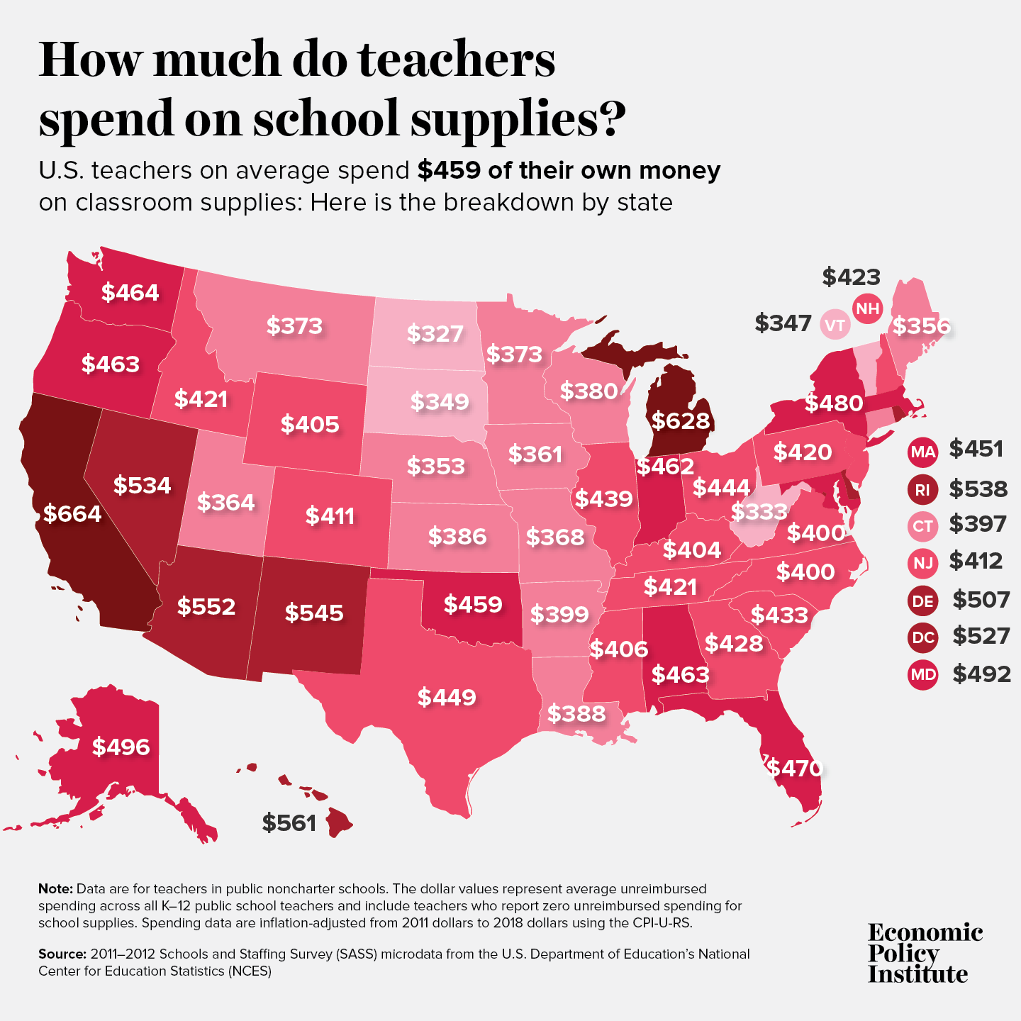
“What’s ahead for teachers in light of the threat of COVID-19 spreading will only add to the existing challenges and stress,” predicts García. “Teachers already act as first respondents when it comes to children’s basic needs, and schools are the only place where some students can have access to hot meals, medical care, washing their dirty laundry, or even to shelter. These, as well as the expense outlays, are worse in schools serving larger shares of low-income students.”Read more
Trump’s payroll tax cuts are a terrible opening bid to address the economic fallout of COVID-19: But employer tax credits can be part of the economic response if they finance direct benefits for workers
Unconditional tax cuts for employers are a terrible policy response to the economic fallout of COVID-19. But employer tax credits that are tied to the provision of specific benefits for workers can be a useful way to deliver emergency help. In the long run, key benefits like paid sick leave and strong unemployment insurance should not rest on employer tax credits, but these credits might be the best way to deliver emergency benefits right now.
The Trump administration has put forward the idea of cutting both employee- and employer-side payroll taxes as the centerpiece of an economic response to the COVID-19 epidemic. This is a terrible opening bid. In late 2010, the Obama White House and a Republican-led Congress agreed on a temporary payroll tax cut for employees only as a compromise measure to provide economic stimulus.
But the employee-side payroll tax cut is an even worse potential compromise this time. One reason is that it would not get enough money out the door and into households’ pockets quickly enough. A COVID-19 recession will come fast and people will need lots of help quickly. A payroll tax cut will dribble out gradually over time. Another reason is the employee-side payroll tax cut is poorly targeted and sends lots of money to high-income households. A COVID-19 recession is laser-targeted at sectors with lots of low-wage workers, and the response should be too. So, even employee-side payroll tax cuts are a poor centerpiece of any policy package responding to the coming slowdown.
Employer-side payroll tax cuts are even much worse. They are a pure windfall to business and would do nothing for workers in the short run. These employer-side cuts should be flatly opposed.
There is, however, a potential role for employer tax credits as a way to stand-up emergency paid sick leave or work sharing or unemployment insurance. The optimal way for these programs to work is to have them be an ongoing part of our social safety net that take effect automatically during downturns. In the case of work-sharing and unemployment insurance, these should be social insurance programs financed in the long run by payroll taxes. Paid sick leave should be a mandated labor standard. But since we do not have strong systems in place to provide these benefits to workers affected by the economic fallout of COVID-19 in the short run, and because placing new costs on employers just as revenue potentially craters might not be optimal, we could use employer tax credits to finance the emergency provision of key benefits like paid sick leave and expanded unemployment insurance.
Economists Jared Bernstein and Jesse Rothstein, for example, have a proposal to use employer tax credits to finance quicker-acting unemployment insurance that allows workers to stay on payroll and be paid even while not working during a COVID-19 downturn. Dean Baker made a similar proposal as the Great Recession loomed.
Policy discussions about buffering the economy from the COVID-19 shock are moving very quickly and lines are being drawn. It remains the case that large direct payments to households and having the federal government pick up states’ Medicaid spending for a year are likely the most valuable macroeconomic support that could be provided because they’re well-targeted to counteract the particular damage inflicted by a COVID-19 recession.
It also remains the case that unconditional employer tax cuts should be rejected flatly as a solution. But there does remain a potential role for employer tax credits in helping deliver benefits to workers. As long as these tax credits are used solely for this purpose, they should be considered.
A Trump attack on government, flying largely under the radar: Trump wants to help corporations suspected of violating the law
Health inspections of cruise ships, to reduce the spread of infections. A recall of flammable infant sleepwear. An order to clean up contaminated soil or water. This work of the federal government often lets us take for granted the safety of the food we eat, the clothes we put on our kids, and even our collective ability to fight new illnesses like the coronavirus.
We can’t take it for granted anymore. An obscure agency that most Americans have never heard of has issued a request for information that one-sidedly solicits input about how government is a problem, with the transparent goal of creating more roadblocks to government enforcement of environmental, consumer protection, labor, and other regulations. Right-wing groups are already mobilizing a campaign in response, prompting scores of comments expressing fervent yet vague support for the president. Many more comments are surely in the works, by corporations offering more polished and pointed explanations of their need to operate unfettered. The Trump administration has made clear its intent to do their bidding and more, but we don’t have to make it easy. Think tanks, public interest lawyers, community and advocacy organizations, and the general public can and should weigh in, to protect the government’s basic ability to protect our shared well-being.
At the hub of the agencies that report to the president is the Office of Management and Budget (OMB), which sets rules across the federal government for what agencies do and how they behave. In late January, the OMB issued a highly unorthodox request that assumes agencies behave unfairly, and asks how to make agency actions friendlier to alleged lawbreakers. It’s a clear invitation to corporate wrongdoers to provide anecdotes masquerading as evidence. The OMB’s head characterized the request as a means to end “bureaucratic bullying.” They’ve already decreed that agencies must repeal two rules for every new one they issue, no matter the harm to the public; this request is another effort to hamstring the government’s ability to pursue corporate wrongdoing.
The OMB’s request strangely floats importing criminal due process concepts into the civil administrative context. It asks whether there should be an “initial presumption of innocence,” for example, and whether investigated parties should be able “to require an agency to ‘show cause’ to continue an investigation.” But we are talking about corporations under civil investigation based on potential harm to broad swaths of people. If a business is suspected of polluting a playground, do we really want to slow down investigation and enforcement? Most of us would prefer swift government action in such circumstances.Read more
Amid COVID-19 outbreak, the workers who need paid sick days the most have the least
The United States is unprepared for the COVID-19 pandemic given that many workers throughout the economy will have financial difficulty in following the CDC’s recommendations to stay home and seek medical care if they think they’ve become infected. Millions of U.S. workers and their families don’t have access to health insurance, and only 30% of the lowest-paid workers have the ability to earn paid sick days—workers who typically have lots of contact with the public and aren’t able to work from home.
There are deficiencies in paid sick days coverage per sector, particularly among those workers with a lot of public exposure. Figure A displays access to paid sick leave by sector. Information and financial activities have the highest rates of coverage at 95% and 91%, respectively. Education and health services, manufacturing, and professional and business services have lower rates of coverage, but still maintain at least three-quarters of workers with access. Trade, transportation, and utilities comes in at 72%, but there are significant differences within that sector ranging from utilities at 95% down to retail trade at 64% (not shown). Over half of private-sector workers in leisure and hospitality do not have access to paid sick days. Within that sector, 55% of workers in accommodation and food services do not have access to paid sick days (not shown).
Workers face stark differences in access to paid sick days, depending on what sector they work in: Share of private-sector workers with access to paid sick days, by sector, 2019
| Sector | Share of workers who with paid sick leave |
|---|---|
| Information | 95% |
| Financial activities | 91% |
| Education and health services | 84% |
| Manufacturing | 79% |
| Professional and business services | 76% |
| Trade, transportation, and utilities | 72% |
| Other services | 59% |
| Construction | 58% |
| Leisure and hospitality | 48% |
Source: U.S. Bureau of Labor Statistics, National Compensation Survey 2019.
Of the public health concerns in the workforce related to COVID-19, two loom large: those who work with the elderly, because of how dangerous the virus is for that population, and those who work with food, because of the transmission of illness. Research shows that more paid sick days is related to reduced flu rates. There is no reason to believe contagion of COVID-19 will be any different. When over half of workers in food services and related occupations do not have access to paid sick days, the illness may spread more quickly.
What exacerbates the lack of paid sick days among these workers is that their jobs are already not easily transferable to working from home. On average, about 29% of all workers can work from home. And, not surprisingly, workers in sectors where they are more likely to have paid sick days are also more likely to be able to work from home. Over 50% of workers in information, financial activities, and professional and business services can work from home. However, only about 9% of workers in leisure and hospitality are able to work from home.
Many of the 73% of workers with access to paid sick days will not have enough days banked to be able to take off for the course of the illness to take care of themselves or a family member. COVID-19’s incubation period could be as long as 14 days, and little is known about how long it could take to recover once symptoms take hold. Figure B displays the amount of paid sick days workers have access to at different lengths of service. Paid sick days increase by years of service, but even after 20 years, only 25% of private-sector workers are offered at least 10 days of paid sick days a year.
The small sliver of green shows that a very small share (only about 4%) of workers—regardless of their length of service—have access to more than 14 paid sick days. That’s just under three weeks for a five-day-a-week worker, assuming they have that many days at their disposal at the time when illness strikes. The vast majority of workers, over three-quarters of all workers, have nine days or less of paid sick time. This clearly shows that even among workers with access to some amount of paid sick days, the amounts are likely to be insufficient.
Sufficient paid sick days provisions in the case of COVID-19 are scarce: Share of workers with access to paid sick days by number of days and length of service
| Access to more than 14 sick days | Access to 10–14 sick days | Access to 5–9 sick days | Access to less than 5 sick days | |
|---|---|---|---|---|
| After one year of service | 3 % | 18% | 54% | 25% |
| After five years of service | 4 | 19 | 54 | 24 |
| After 10 years of service | 4 | 19 | 54 | 23 |
| After 20 years of service | 4 | 19 | 54 | 23 |
Source: U.S. Bureau of Labor Statistics, National Compensation Survey 2019
Getting serious about the economic response to COVID-19
With the stock market plummeting and hysteria around COVID-19 (commonly known as the coronavirus) escalating, it is time to get serious about the economic policy response. Policymakers and the public will need help in distinguishing between smart responses and those that are just ideological opportunism, such as calls for cuts in taxes and regulations, for example.
Simply put, smart responses must be tailored to the type of recession the outbreak could cause if policymakers don’t act.
The three key elements of a potential COVID-19 recession are:
- If it comes, it will come fast.
- It will hit lower-wage workers first and hardest.
- It will impose even faster and larger costs on state and local governments than recessions normally do.
Each one of these should be targeted directly.
Any economic relief package should come online quickly, it should be even more targeted to help lower-wage workers than usual, and it should rapidly boost state and local government capacity on both the public health and economic fronts. Below I sketch out why these characteristics of the COVID-19 slowdown are likely, and what a tailored response to each would be.
First, if the COVID-19 outbreak slows the economy, it could happen very rapidly. This is quite different, for example, than the onset of the Great Recession. That recession was caused by the bursting of the home price bubble, which essentially began in mid-2006. From that point on the recession was near-inevitable, but it took literally years to gather steam. As the Great Recession loomed, the key characteristics policymakers should have demanded of any proposed stimulus package should have been: effective, large, and sustained. Fiscal policymakers decisively failed on the last point, and dwindling fiscal support hampered recovery for years.
A COVID-19 driven recession would be quite different in that it would hit quickly. The spread of the disease has been quite rapid in each country it has affected. Further, the public health response to maintain “social distancing” to thwart its spread tends to take effect rapidly as well. Even before the reported cases in the U.S. have reached large numbers, the news are full of cascading cancellations of business and entertainment gatherings. We are almost certainly already feeling the economic effects of the COVID-19 slowdown—it just has not appeared in economic statistics yet (since these statistics tend to appear with a small lag).Read more
Even HBO’s John Oliver didn’t provide the full context on ‘Medicare for All’ and jobs
There’s a lot of rhetoric out there right now about how providing “Medicare for All” (M4A) could destroy the economy or lead to ruinous tax increases. But one bright spot was HBO host John Oliver’s monologue on the plan that went viral last month.
Oliver took a characteristically in-depth look at the issues and was largely positive about how M4A could help a “badly broken” health care system given the millions of people who are uninsured and underinsured. Crucially, he noted that we’re going to pay for health care one way or the other, and M4A largely doesn’t add to the costs we pay (indeed, it could well reduce them significantly in the long run), instead it just changes how we pay these costs—substituting taxes for premiums.
Oliver provided a comprehensive accounting of the benefits of the health care proposal, but he also raised some possible pitfalls, including the jobs that could be lost given the elimination of the private health insurance industry. The problem is he quoted a 1.8 million job-loss figure that’s been widely circulated but is widely misleading when presented without context, as I explain in my new analysis of M4A’s impact on the labor market.