Income Stagnation in 2014 Shows the Economy Is Not Working for Most Families
We learned from the Census Bureau this morning that the decent employment growth in 2014 yielded no improvements in wages and, not surprisingly, no improvement in the median incomes of working-age households or drop in the number of people living in poverty. Wage trends greatly determine how fast incomes at the middle and bottom grow, as well as the overall path of income inequality, as we argued in Raising America’s Pay. This is for the simple reason that most households, including those with low incomes, rely on labor earnings for the vast majority of their income.
The Census data show that from 2013–2014, median household income for non-elderly households (those with a head of household younger than 65 years old) decreased 1.3 percent from $61,252 to $60,462. This decrease unfortunately exacerbates the trend of losses incurred during the Great Recession and the losses that prevailed in the prior business cycle from 2000–2007. Median household income for non-elderly households in 2014 ($60,462) was 9.2 percent, or $6,113, below its level in 2007. The disappointing trends of the Great Recession and its aftermath come on the heels of the weak labor market from 2000–2007, during which the median income of non-elderly households fell significantly from $68,941 to $66,575, the first time in the post-war period that incomes failed to grow over a business cycle. Altogether, from 2000–2014, the median income for non-elderly households fell from $68,941 to $60,462, a decline of $8,479, or 12.3 percent.
Real median household income, all and non-elderly, 1995–2014
| All households | All households- imputed series | All households- new series | Non-elderly households | Non-elderly households- imputed series | Non-elderly households- new series | |
|---|---|---|---|---|---|---|
| 1995-01-01 | $52,555 | $54,231 | $60,378 | $62,268 | ||
| 1996-01-01 | $53,319 | $55,020 | $61,506 | $63,431 | ||
| 1997-01-01 | $54,417 | $56,152 | $62,298 | $64,248 | ||
| 1998-01-01 | $56,394 | $58,193 | $64,823 | $66,852 | ||
| 1999-01-01 | $57,815 | $59,659 | $66,493 | $68,575 | ||
| 2000-01-01 | $57,718 | $59,559 | $66,849 | $68,941 | ||
| 2001-01-01 | $56,460 | $58,261 | $65,819 | $67,879 | ||
| 2002-01-01 | $55,801 | $57,580 | $65,145 | $67,184 | ||
| 2003-01-01 | $55,752 | $57,530 | $64,573 | $66,594 | ||
| 2004-01-01 | $55,558 | $57,330 | $63,816 | $65,814 | ||
| 2005-01-01 | $56,172 | $57,963 | $63,399 | $65,384 | ||
| 2006-01-01 | $56,589 | $58,394 | $64,250 | $66,261 | ||
| 2007-01-01 | $57,348 | $59,177 | $64,554 | $66,575 | ||
| 2008-01-01 | $55,303 | $57,067 | $62,436 | $64,391 | ||
| 2009-01-01 | $54,933 | $56,685 | $61,603 | $63,532 | ||
| 2010-01-01 | $53,497 | $55,203 | $60,012 | $61,890 | ||
| 2011-01-01 | $52,680 | $54,360 | $58,559 | $60,392 | ||
| 2012-01-01 | $52,595 | $54,272 | $59,127 | $60,978 | ||
| 2013-01-01 | $52,779 | $54,462 | $54,462 | $59,393 | $61,252 | $61,252 |
| 2014-01-01 | $53,657 | $60,462 |

Note: CPS ASEC changed its methodology for data years 2013 and 2014, hence the break in the series in 2013. Solid lines are actual CPS ASEC data; dashed lines denote historical values imputed by applying the new methodology to past income trends. Non-elderly households are those in which the head of household is younger than age 65. Shaded areas denote recessions.
To account for the redesign of the CPS ASEC survey, when the difference between the original data for 2013 and the redesigned data for 2013 is small in magnitude (less than a 1 percent difference) and statistically insignificantly different, data for 2013 is an average of the original and redesigned data. When the difference between them is relatively large in magnitude (1 percent or greater) or statistically significantly different, we display a break in the series and impute the ratio between them to historical data.
Source: EPI analysis of Current Population Survey Annual Social and Economic Supplement Historical Income Tables (Tables H-5 and HINC-02)
What to Watch in the Census Poverty and Income Data
On Wednesday, the Census Bureau will release the latest data on income, poverty, and health insurance coverage. As EPI’s research team eagerly awaits this release, there are a few things we will be watching for.
Due to a redesign of the underlying survey (the Current Population Survey Annual Social and Economic Supplement, or CPS ASEC) in 2014, current estimates of incomes and poverty will not be directly comparable to years prior to 2013. This will also be a problem, albeit to a much lesser extent, with data on labor earnings. Since the Census Bureau will provide 2013 estimates based on both the old survey and the redesigned survey, we plan to deal with the break in the data series by focusing on two time periods. The first time period will cover 2000–2013, based on estimates from the old survey format. The second will be based on the redesigned estimates for 2013–2014. While in much of our analysis we will impute recent changes onto the data back to 2000 to get a better sense in that longer term trend, we will provide clear guidance on how the survey redesign affects these trends.
On Wednesday, we are going to most closely examine median earnings for men and women, median household income, and poverty rates. We will be looking not only at what we expect to be some improvement in these metrics between 2013 and 2014, but also what’s been happening since 2000. We know that even in the full business cycle 2000-07, earnings and incomes never fully recovered pre-recession peaks, and when the Great Recession hit, the economic impacts were devastating for many. To the extent the data will allow, we will look at how much the recovery has helped improve the economic lot for Americans, with particular attention to livelihood across racial and ethnic groups.
There’s More to Economic Security than the Official Poverty Measure
Next week, the Census Bureau will release its estimates of the number of Americans who lived in poverty in 2014. The official poverty measure is an important metric—particularly since it’s been in place for nearly 50 years, and its measurement methodology hasn’t had major revisions over that time. As shown in the figure below, the share of Americans living at or below the official poverty line fell in the 1960s and stayed within a small range over the last four decades or so, generally rising in recessions and falling in expansions. Since 2000, the official poverty rate has seen a lot more up than down—the poverty rate at the end of the business cycle in 2007 was higher than at the beginning. 2013 was the first year the poverty rate turned the corner and saw some meaningful improvement since the start of the Great Recession. On Wednesday, September 16, we will see whether that progress has continued. While it would be great to see reductions in poverty over the last year, the fact is had economic growth over the last four decades been broadly shared, we could have made much more progress in reducing poverty, rather than just treading water.
Poverty rate, 1959–2013
| Actual poverty rate | |
|---|---|
| 1959-01-01 | 22.4% |
| 1960-01-01 | 22.2% |
| 1961-01-01 | 21.9% |
| 1962-01-01 | 21.0% |
| 1963-01-01 | 19.5% |
| 1964-01-01 | 19.0% |
| 1965-01-01 | 17.3% |
| 1966-01-01 | 14.7% |
| 1967-01-01 | 14.2% |
| 1968-01-01 | 12.8% |
| 1969-01-01 | 12.1% |
| 1970-01-01 | 12.6% |
| 1971-01-01 | 12.5% |
| 1972-01-01 | 11.9% |
| 1973-01-01 | 11.1% |
| 1974-01-01 | 11.2% |
| 1975-01-01 | 12.3% |
| 1976-01-01 | 11.8% |
| 1977-01-01 | 11.6% |
| 1978-01-01 | 11.4% |
| 1979-01-01 | 11.7% |
| 1980-01-01 | 13.0% |
| 1981-01-01 | 14.0% |
| 1982-01-01 | 15.0% |
| 1983-01-01 | 15.2% |
| 1984-01-01 | 14.4% |
| 1985-01-01 | 14.0% |
| 1986-01-01 | 13.6% |
| 1987-01-01 | 13.4% |
| 1988-01-01 | 13.0% |
| 1989-01-01 | 12.8% |
| 1990-01-01 | 13.5% |
| 1991-01-01 | 14.2% |
| 1992-01-01 | 14.8% |
| 1993-01-01 | 15.1% |
| 1994-01-01 | 14.5% |
| 1995-01-01 | 13.8% |
| 1996-01-01 | 13.7% |
| 1997-01-01 | 13.3% |
| 1998-01-01 | 12.7% |
| 1999-01-01 | 11.9% |
| 2000-01-01 | 11.3% |
| 2001-01-01 | 11.7% |
| 2002-01-01 | 12.1% |
| 2003-01-01 | 12.5% |
| 2004-01-01 | 12.7% |
| 2005-01-01 | 12.6% |
| 2006-01-01 | 12.3% |
| 2007-01-01 | 12.5% |
| 2008-01-01 | 13.2% |
| 2009-01-01 | 14.3% |
| 2010-01-01 | 15.1% |
| 2011-01-01 | 15.0% |
| 2012-01-01 | 15.0% |
| 2013-01-01 | 14.5% |
Source: EPI analysis of Current Population Survey Annual Social and Economic Supplement Historical Poverty Tables (Tables 2 and 4), Bureau of Economic Analysis National Income Product Accounts public data, and Danziger and Gottschalk (1995)
H-2B Wage Rule Loophole Lets Employers Exploit Migrant Workers
Last week the New York Times reported the latest innovation from employers who use the H-2B visa temporary foreign worker program to hire workers to staff traveling carnivals (think your local county or state fair): an employer-created union that collectively bargains with employers on behalf of workers to keep wages artificially low. Thanks to a loophole in H-2B wage regulations, low-wage, low-road employers are permitted to pay their temporary foreign workers dreadfully low wages.
The genesis of the prevailing wage loophole
For about half a decade, thanks to an H-2B wage regulation the George W. Bush administration illegally put in place in 2008, employers of landscapers, dishwashers, tree planters, maids, janitors, carnival workers, and construction workers were allowed to pay their H-2B employees as little as the local 17th percentile wage. (This is legally defined as the “Level 1” prevailing wage, based on Labor Department wage survey data for the job and local area.) After the rule was struck down in federal court in 2010, the Obama administration promulgated a final wage rule in 2011 that would have required employers to pay H-2B workers the local average wage (what’s also known as the Level 3 prevailing wage). However, this effort led to years of federal litigation brought by H-2B employers that stopped the rule in its tracks, and spurred an onslaught of corporate lobbying that convinced members of Congress from both major parties to deny funding to the Labor Department to enforce the rule.
Finally, in April 2013, the wage rule for the H-2B program was re-promulgated as an interim final rule issued jointly by the departments of Labor and Homeland Security. (The fact that the rule was issued jointly negated the main legal challenge, namely that the Labor Department lacked authority to promulgate any H-2B wage regulation.) The 2008 and 2013 H-2B wage rules both required employers to pay their H-2B employees the wage set out in an applicable collective bargaining agreement (CBA). But under the 2008 rule, if no CBA applied, then employers were allowed to pay the 17th percentile wage. The 2011 final H-2B wage rule that Congress blocked would have required employers to pay the higher wage between the CBA wage or the local average wage. Under the 2013 rule, if no CBA covered the H-2B worker, then the employer would have to pay the local average wage.
JOLTS Report is Evidence of an Economy Moving Sideways
Today’s Job Openings and Labor Turnover Survey (JOLTS) report corroborates last week’s jobs report, which continued to provide evidence that the economy is at best moving at a slow jog, with meager wage growth and employment growth that’s just keeping up with the growth in the working age population. The rate of job openings increased in July, while the hires rate fell and the quits rate remains depressed.
There continues to be a significant gap between the number of people looking for jobs and the number of job openings. The figure below illustrates the overall improvement in the economy over the last five years, as the unemployment level continues to fall and job openings rise. In a tighter economy (like the one shown in the initial year of data), these levels would be much closer together. So it’s clear that there is still a significant amount slack in the economy. Furthermore, on top of the 8+ million unemployed workers warming the bench, there are still more than three million workers sitting in the stands with little hope to even get in the game.
Job openings levels and unemployment levels, December 2000-July 2015
| Month | Job Openings level | Unemployment level |
|---|---|---|
| Dec-2000 | 4.934 | 5.634 |
| Jan-2001 | 5.273 | 6.023 |
| Feb-2001 | 4.706 | 6.089 |
| Mar-2001 | 4.618 | 6.141 |
| Apr-2001 | 4.668 | 6.271 |
| May-2001 | 4.444 | 6.226 |
| Jun-2001 | 4.232 | 6.484 |
| Jul-2001 | 4.354 | 6.583 |
| Aug-2001 | 4.095 | 7.042 |
| Sep-2001 | 3.973 | 7.142 |
| Oct-2001 | 3.594 | 7.694 |
| Nov-2001 | 3.545 | 8.003 |
| Dec-2001 | 3.586 | 8.258 |
| Jan-2002 | 3.587 | 8.182 |
| Feb-2002 | 3.412 | 8.215 |
| Mar-2002 | 3.605 | 8.304 |
| Apr-2002 | 3.357 | 8.599 |
| May-2002 | 3.525 | 8.399 |
| Jun-2002 | 3.325 | 8.393 |
| Jul-2002 | 3.343 | 8.39 |
| Aug-2002 | 3.462 | 8.304 |
| Sep-2002 | 3.319 | 8.251 |
| Oct-2002 | 3.502 | 8.307 |
| Nov-2002 | 3.585 | 8.52 |
| Dec-2002 | 3.074 | 8.64 |
| Jan-2003 | 3.686 | 8.52 |
| Feb-2003 | 3.402 | 8.618 |
| Mar-2003 | 3.101 | 8.588 |
| Apr-2003 | 3.182 | 8.842 |
| May-2003 | 3.201 | 8.957 |
| Jun-2003 | 3.356 | 9.266 |
| Jul-2003 | 3.195 | 9.011 |
| Aug-2003 | 3.239 | 8.896 |
| Sep-2003 | 3.054 | 8.921 |
| Oct-2003 | 3.196 | 8.732 |
| Nov-2003 | 3.316 | 8.576 |
| Dec-2003 | 3.334 | 8.317 |
| Jan-2004 | 3.391 | 8.37 |
| Feb-2004 | 3.437 | 8.167 |
| Mar-2004 | 3.42 | 8.491 |
| Apr-2004 | 3.466 | 8.17 |
| May-2004 | 3.658 | 8.212 |
| Jun-2004 | 3.384 | 8.286 |
| Jul-2004 | 3.835 | 8.136 |
| Aug-2004 | 3.578 | 7.99 |
| Sep-2004 | 3.704 | 7.927 |
| Oct-2004 | 3.779 | 8.061 |
| Nov-2004 | 3.456 | 7.932 |
| Dec-2004 | 3.846 | 7.934 |
| Jan-2005 | 3.595 | 7.784 |
| Feb-2005 | 3.842 | 7.98 |
| Mar-2005 | 3.891 | 7.737 |
| Apr-2005 | 4.115 | 7.672 |
| May-2005 | 3.824 | 7.651 |
| Jun-2005 | 4.018 | 7.524 |
| Jul-2005 | 4.162 | 7.406 |
| Aug-2005 | 4.085 | 7.345 |
| Sep-2005 | 4.227 | 7.553 |
| Oct-2005 | 4.23 | 7.453 |
| Nov-2005 | 4.341 | 7.566 |
| Dec-2005 | 4.249 | 7.279 |
| Jan-2006 | 4.278 | 7.064 |
| Feb-2006 | 4.308 | 7.184 |
| Mar-2006 | 4.537 | 7.072 |
| Apr-2006 | 4.495 | 7.12 |
| May-2006 | 4.432 | 6.98 |
| Jun-2006 | 4.331 | 7.001 |
| Jul-2006 | 4.081 | 7.175 |
| Aug-2006 | 4.411 | 7.091 |
| Sep-2006 | 4.498 | 6.847 |
| Oct-2006 | 4.454 | 6.727 |
| Nov-2006 | 4.622 | 6.872 |
| Dec-2006 | 4.552 | 6.762 |
| Jan-2007 | 4.59 | 7.116 |
| Feb-2007 | 4.481 | 6.927 |
| Mar-2007 | 4.657 | 6.731 |
| Apr-2007 | 4.534 | 6.85 |
| May-2007 | 4.531 | 6.766 |
| Jun-2007 | 4.639 | 6.979 |
| Jul-2007 | 4.43 | 7.149 |
| Aug-2007 | 4.508 | 7.067 |
| Sep-2007 | 4.481 | 7.17 |
| Oct-2007 | 4.278 | 7.237 |
| Nov-2007 | 4.278 | 7.24 |
| Dec-2007 | 4.323 | 7.645 |
| Jan-2008 | 4.223 | 7.685 |
| Feb-2008 | 4.039 | 7.497 |
| Mar-2008 | 4.012 | 7.822 |
| Apr-2008 | 3.85 | 7.637 |
| May-2008 | 4 | 8.395 |
| Jun-2008 | 3.67 | 8.575 |
| Jul-2008 | 3.762 | 8.937 |
| Aug-2008 | 3.584 | 9.438 |
| Sep-2008 | 3.21 | 9.494 |
| Oct-2008 | 3.273 | 10.074 |
| Nov-2008 | 3.059 | 10.538 |
| Dec-2008 | 3.049 | 11.286 |
| Jan-2009 | 2.763 | 12.058 |
| Feb-2009 | 2.794 | 12.898 |
| Mar-2009 | 2.493 | 13.426 |
| Apr-2009 | 2.271 | 13.853 |
| May-2009 | 2.413 | 14.499 |
| Jun-2009 | 2.388 | 14.707 |
| Jul-2009 | 2.146 | 14.601 |
| Aug-2009 | 2.294 | 14.814 |
| Sep-2009 | 2.434 | 15.009 |
| Oct-2009 | 2.376 | 15.352 |
| Nov-2009 | 2.419 | 15.219 |
| Dec-2009 | 2.49 | 15.098 |
| Jan-2010 | 2.706 | 15.046 |
| Feb-2010 | 2.561 | 15.113 |
| Mar-2010 | 2.652 | 15.202 |
| Apr-2010 | 3.097 | 15.325 |
| May-2010 | 2.9 | 14.849 |
| Jun-2010 | 2.728 | 14.474 |
| Jul-2010 | 2.929 | 14.512 |
| Aug-2010 | 2.869 | 14.648 |
| Sep-2010 | 2.782 | 14.579 |
| Oct-2010 | 3.026 | 14.516 |
| Nov-2010 | 3.072 | 15.081 |
| Dec-2010 | 2.909 | 14.348 |
| Jan-2011 | 2.917 | 14.046 |
| Feb-2011 | 3.065 | 13.828 |
| Mar-2011 | 3.132 | 13.728 |
| Apr-2011 | 3.099 | 13.956 |
| May-2011 | 3.032 | 13.853 |
| Jun-2011 | 3.194 | 13.958 |
| Jul-2011 | 3.417 | 13.756 |
| Aug-2011 | 3.138 | 13.806 |
| Sep-2011 | 3.557 | 13.929 |
| Oct-2011 | 3.422 | 13.599 |
| Nov-2011 | 3.215 | 13.309 |
| Dec-2011 | 3.527 | 13.071 |
| Jan-2012 | 3.653 | 12.812 |
| Feb-2012 | 3.517 | 12.828 |
| Mar-2012 | 3.837 | 12.696 |
| Apr-2012 | 3.627 | 12.636 |
| May-2012 | 3.696 | 12.668 |
| Jun-2012 | 3.785 | 12.688 |
| Jul-2012 | 3.587 | 12.657 |
| Aug-2012 | 3.637 | 12.449 |
| Sep-2012 | 3.614 | 12.106 |
| Oct-2012 | 3.729 | 12.141 |
| Nov-2012 | 3.741 | 12.026 |
| Dec-2012 | 3.64 | 12.272 |
| Jan-2013 | 3.77 | 12.497 |
| Feb-2013 | 4.023 | 11.967 |
| Mar-2013 | 3.891 | 11.653 |
| Apr-2013 | 3.84 | 11.735 |
| May-2013 | 3.829 | 11.671 |
| Jun-2013 | 3.864 | 11.736 |
| Jul-2013 | 3.829 | 11.357 |
| Aug-2013 | 3.893 | 11.241 |
| Sep-2013 | 3.955 | 11.251 |
| Oct-2013 | 4.076 | 11.161 |
| Nov-2013 | 4.073 | 10.814 |
| Dec-2013 | 3.977 | 10.376 |
| Jan-2014 | 3.906 | 10.28 |
| Feb-2014 | 4.160 | 10.387 |
| Mar-2014 | 4.210 | 10.384 |
| Apr-2014 | 4.417 | 9.696 |
| May-2014 | 4.608 | 9.761 |
| Jun-2014 | 4.710 | 9.453 |
| Jul-2014 | 4.726 | 9.648 |
| Aug-2014 | 4.925 | 9.568 |
| Sep-2014 | 4.678 | 9.237 |
| Oct-2014 | 4.849 | 8.983 |
| Nov-2014 | 4.886 | 9.071 |
| Dec-2014 | 4.877 | 8.688 |
| Jan-2015 | 4.965 | 8.979 |
| Feb-2015 | 5.144 | 8.705 |
| Mar-2015 | 5.109 | 8.575 |
| Apr-2015 | 5.334 | 8.549 |
| May-2015 | 5.357 | 8.674 |
| Jun-2015 | 5.323 | 8.299 |
| Jul-2015 | 5.753 | 8.266 |
Note: Shaded areas denote recessions.
Source: EPI analysis of Bureau of Labor Statistics Job Openings and Labor Turnover Survey and Current Population Survey
Will Republicans Cut Budgets for Worker Safety, Pension Protection, and Wage and Hour Enforcement?
The White House sent a Labor Day message from Director of the Office of Management and Budget Shaun Donovan about the many important issues affecting working Americans that will be decided in the next month of congressional budget negotiations. The message is well worth reading.
Donovan describes what he calls a “double-pronged attack on the workers we are celebrating today.” This attack includes deep cuts at the Wage and Hour Division, which protects workers against wage theft by crooked employers, and which collected $250 million in back pay for workers last year. Republicans also want limits on the use of third-party experts to accompany OSHA compliance officers on workplace safety inspections, where they can point out hazards OSHA might miss. They want to cut the budget and limit enforcement of the National Labor Relations Board’s rules to protect workers who join together for better working conditions. They want to block a new OSHA rule that will save thousands of workers from death, disabling lung disease, or cancer from inhaling silica dust. And they are trying to kill a new effort by the Department of Labor to protect retirees from financial advisors who put their own interests ahead of their clients’ interests.
None of the laws protecting working Americans from wage theft, on-the-job injury, unlawful retaliation, or self-dealing by financial advisors is meaningful if the government doesn’t enforce them. That takes resources and staff—investigators and lawyers who can take on big corporations or reckless businesses. Yet congressional Republicans want to cut funding for enforcement of all these laws. At OSHA, for example, Republicans want a 10 percent cut—$57 million, even though OSHA’s inspectors already can’t get to even one percent of workplaces in a year, and negligent employers put workers in harm’s way every day and kill nearly 100 employees a week.
Fisher II—Could a Surprise be in Store?
This post originally appeared on SCOTUSblog, as part of a symposium on Fisher v. University of Texas at Austin, the challenge to the university’s use of affirmative action in its undergraduate admissions process.
The Supreme Court’s affirmative action decisions have been suffused with hypocrisy. Justice Ruth Bader Ginsburg called them out, with barely more gentle phrasing, in her lone dissent to the seven-to-one majority opinion the first time Fisher v. University of Texas at Austin (2013) was before the Court. “Only an ostrich,” she observed, “could regard the supposedly neutral alternatives as race unconscious,” and only a (contorted) legal mind “could conclude that an admissions plan designed to produce racial diversity is not race conscious.”
The “diversity” standard in college admissions has gained great popularity because advocates of race-based affirmative action, stymied by the Court since Regents of the University of California v. Bakke, latched onto it as an alternative that could satisfy strict scrutiny. Many proponents have since persuaded themselves that diversity is, after all, a better approach than race-based affirmative action and that if the Court had not required it, we would have had to invent it. Yet while diversity in college classes is certainly an important educational and social goal, its elevation nonetheless dodges the nation’s racial legacy and avoids our constitutional and moral obligation to remedy the effects of centuries of slavery and legally sanctioned segregation. Without acknowledging we were doing so, we have engaged in a legal sleight of hand, substituting enriching the educational experience for remedying past injustice in designing affirmative action policy.
Underlying all this has been the Court majority’s conviction, most recently in Fisher I, that university officials have not identified specific Fourteenth Amendment violations for which their policies are a remedy, and therefore their consideration of race injects, without constitutional justification, a discriminatory racial consideration into the admissions process. The paucity of African Americans at the University of Texas reflects no de jure exclusion, the Fisher I majority believed, but only de factosocial inequality for which there is no race-conscious constitutional remedy. Therefore, including racial diversity in a scheme of skill-based, interest-based, or economic diversity is suspect, requiring very strict scrutiny. Indeed, the conditions set by the Fisher I majority opinion suggest a scrutiny that is strict in theory but fatal in fact. (I discuss the Fisher cases here only as they relate to the treatment of African Americans in affirmative action plans, not to that of other national or ethnic minorities or of disadvantaged economic groups; each has a different history and status, requires different opportunities to succeed, and raises different social policy and constitutional concerns).
African American Youth Experienced the Largest Boost in Summer Labor Force Participation and Employment
As students head back to school this fall, today’s release of the August jobs numbers provides the first complete look at the summer job market for teens. As a whole, the stronger start to the 2015 summer jobs season (compared to last summer) signaled by the June youth employment numbers was sustained throughout the summer. According to seasonally unadjusted teen employment-to-population (EPOP) ratios, averaged for the months of June, July and August, African American youth experienced the largest boost to summer employment compared to last year. Summer employment was up 2.5 percentage points for black teens, compared to a 1.5 percentage point increase for Hispanic youth and a 1.2 percentage point increase for white teens, as shown in the figure below. Though black teens continue to have the lowest rates of employment, the 2015 summer youth employment rate for black teens was closer to its 2007 pre-Great Recession rate than were those of white and Hispanic youth.
Average teenage (16-19 years) summer employment to population ratio, 2007,2014, and 2015
| 2007 | 2014 | 2015 | |
|---|---|---|---|
| white | 43.9 | 34.3 | 35.5 |
| black | 23.0 | 19.3 | 21.8 |
| hispanic | 31.0 | 25.0 | 26.5 |
Source: EPI analysis of Current Population Survey
The Bottom Line of this Jobs Report: The Fed Should Hold the Line and Let the Economy Continue to Recover
The official unemployment rate (the U3) is only one data point—one that doesn’t include workers who have left the labor force because of weak opportunities or workers who want to be working full-time but can only get part-time work. The fact is that the economy is still not adding jobs fast enough, and the recovery is not creating strong wage growth. The best advice is for the Federal Reserve to continue doing what they’re rightfully doing—keeping rates low to let the economy recovery. Many pundits have been quick to encourage the Federal Reserve to raise rates, but a close look at the data shows that the economy still needs time to grow.
Nonfarm payroll employment rose by only 173,000 in August. While it’s best not to read too much into one month’s data, this brings average monthly job growth down to 212,000 so far in 2015. 2014 saw faster jobs growth: an average of 260,000. By that measure alone, we aren’t seeing an accelerating recovery. In fact, at this slower rate of growth, a full jobs recovery is still two years away.
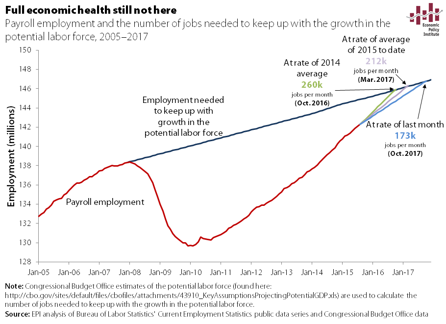
A great example of just how slow this job recovery is going is the flat prime-age employment-to-population ratio (EPOP). This means the economy is only adding enough jobs to keep up with prime-age population growth—nothing more, nothing less. It means the economy is moving at a pace where we are not working off any of the joblessness that remains from the Great Recession. The prime-age EPOP in August (77.2 percent) is still below the lowest trough of the last two recessions (78.1 percent). We have a long way to go before this data point says recovery.
Why a Pro-Worker Agenda is an Anti-Poverty Agenda
This blog post originally appeared on TalkPoverty.org.
Labor Day is a time to honor America’s workers and their contributions to our economy. It is also a time to reflect upon the state of workers’ economic position, and how that position has faltered in recent decades. Except for a short period of across-the-board wage growth in the late 1990s, 2015 marks a general 36-year trend of broad-based wage stagnation and rising inequality in our country, which has had real, adverse effects on low- and middle-income households. This anemic wage growth is closely tied to the stalled progress in reducing poverty since 1979, as many poor people work and their incomes are increasingly dependent upon work. Therefore, along with strengthening the safety net, the goals of anti-poverty advocates should be one in the same with pro-worker advocates: to reverse the decades-long trend of wage stagnation and promote real wage growth for all Americans.
Despite dramatic gains in educational attainment, wages have failed to grow for those at the bottom (and middle) over the last four decades. At the same time, low income household incomes have become increasingly dependent on wages. The figure below shows the major sources of income for non-elderly households in the bottom fifth of the income distribution from 1979 to 2011, using the CBO’s measure of comprehensive income. It shows that incomes of the bottom fifth are increasingly dependent on ties to the workforce. Wages, employer-provided benefits, and tax credits that are dependent on work (such as the EITC) made up 68.3 percent of non-elderly bottom-fifth incomes in 2011, compared with only 58.2 percent in 1979. While government in-kind benefits from sources such as the Supplemental Nutrition Assistance Program (formerly food stamps) and Medicaid increased from 13.2 percent of these bottom-fifth incomes in 1979, to 19.5 percent in 2011, cash transfers such as welfare payments have declined 9.2 percentage points (from 18.6 percent to 9.4 percent).