Summary
The Republican-led effort to repeal the Affordable Care Act (ACA) includes two large fiscal changes: a tax cut and a spending cut.1 Because the U.S. economy still has some productive slack, these significant fiscal changes will affect the pace of economic growth. Essentially, this productive slack is caused by households, businesses, and governments that are still spending less than what the economy could produce if all resources (including workers) were fully employed. This shortfall in spending (or aggregate demand) is hence the current binding constraint on the economy’s growth rate. In this environment, the sudden withdrawal of spending from the economy from ACA repeal would add job loss to the loss of health and financial security for tens of millions of Americans.
This report provides a rough estimate of how the combination of tax cuts and spending cuts in the ACA repeal will affect employment in U.S. states.2 Its main findings are:
- ACA repeal would cut federal spending nationwide by roughly $109 billion in 2019 and taxes by roughly $70 billion in 2019.
- The combination of tax cuts and spending cuts embedded in ACA repeal would reduce national job growth by almost 1.2 million in 2019, all else equal. That is because the spending cuts would hurt job growth more than the tax cuts would help it. The benefit cuts would come mostly out of the pockets of cash-constrained households that will be likely to significantly cut back their spending in response to lower disposable income, while the tax cuts would disproportionately go to high-income households who tend to save a significant portion of increases in disposable income.
- The jobs that would be lost are not just health care jobs. Previous high-quality studies of the jobs gained through Medicaid expansions in the American Recovery and Reinvestment Act (ARRA) indicate that more than three-fourths of the jobs gained were not in the health care sector.
- Every state would lose jobs. How significant this job loss is would be determined by the extent to which a state expanded spending (and thus how much spending it will lose), what portion of a state’s households fall in the groups getting the largest tax cuts (how much it will gain).
- The top 15 job-losing states, as measured by jobs lost as a share of both the total employment and the share of residents under age 65, are Arizona, Colorado, Kentucky, Louisiana, Maryland, Montana, Nevada, New Jersey, New Mexico, North Carolina, Oregon, Rhode Island, Vermont, Washington, and West Virginia.
- Monetary policy is unlikely to be able to provide an expansionary boost to economic activity anywhere near large enough to counteract the significant fiscal contraction posed by ACA repeal, even in 2019. Thus, any claims that any ACA job losses would be neutralized by countervailing Federal Reserve policy are unconvincing.
- States can also be ranked by their relative income burden stemming from ACA repeal. This relative burden measure looks at gains stemming from tax cuts minus losses stemming from spending cuts, scaled to each state’s share of the under-65 population. This population is chosen as our scalar because the coverage expansions of the ACA were aimed entirely at the under-65 population (as the 65 and over population is covered by America’s large single-payer health system, Medicare). Generally, states that took up the ACA Medicaid expansion see a higher relative burden, as they have more to lose from repeal. Additionally, states with a low share of national top 1 percent households will also see a higher relative burden, as they will receive lower-than-average benefits from the tax cuts embedded in ACA repeal.
- While states that never took up the Medicaid expansions that were part of ACA generally face a lower relative burden from repeal, it is important to note that these same states benefit disproportionately from the insurance premium and cost-sharing subsidies of the ACA. Overall, insurance premium and cost-sharing subsidies are roughly 0.4 percent of non-expansion states’ gross domestic product (GDP), while they are roughly 0.15 percent of GDP in expansion states.
Likely fiscal impacts of ACA repeal
Health insurance coverage expanded under the ACA due to two main features: a large expansion of the existing Medicaid program and subsidies that help households afford insurance coverage in the individual (nongroup) market.3 The Medicaid expansions are tightly targeted to the poorest households—those with incomes below 138 percent of the federal poverty level. The premium subsidies for nongroup insurance purchase are available to households making up to 400 percent of the federal poverty level, but are progressive and are much more generous for those making up to 250 percent of the federal poverty level. For households making up to 250 percent of the federal poverty level, substantial subsidies are also offered to help cover cost-sharing expenses (out-of-pocket costs such as co-payments).
These coverage expansions are financed in part by tax increases. The bulk of these tax increases are extraordinarily progressive, i.e., they fall heavily on high-income households. The ACA instituted a 0.9 percent surtax on individual earnings above $200,000. Further, the 3.8 percent Medicare tax rate applying to these high individual earnings was also extended to most forms of capital (investment) income at the household level (with a higher threshold for non-single filers). These progressive tax increases account for roughly 80 percent of the new taxes imposed by the ACA.
Other tax increases used to finance the ACA coverage expansions were smaller, but also less progressive. For example, excise taxes were imposed on large employers (those with over 50 full-time equivalent employees) that did not offer qualified, affordable insurance to workers and on individuals who did not obtain coverage.
Blumberg, Buettgens, and Holahan (2016) have estimated the likely impact of ACA repeal on the spending flows that financed coverage expansions for each state. They assume that full ACA repeal occurs in 2019, and then provide state-by-state estimates of how much Medicaid spending, premium subsidies, and cost-sharing subsidies will be reduced due to that repeal.
The Tax Policy Center (TPC) has estimated the distributional impact of tax cuts related to ACA repeal at the national level, i.e., the share of tax cuts going to households of different income levels.4 Their data indicate that an extraordinary 57.4 percent of these tax cuts would accrue to the top 1 percent, with over a third accruing to the top 0.1 percent alone. To assign the incidence (division) of these tax cuts across states we use two data sources. First, we calculate the distribution of households by state that fall into nationally defined income fifths using data from the American Community Survey (ACS). To get further texture on the distribution of the (national) top 1 percent and 10 percent of households across states, we use data provided by Frank (2017). We use this information from the ACS and Frank (2017) to allocate the share of ACA tax cuts that accrue to each state.
Table 1 sums up this information. The first set of data columns show the dollar value of cuts in Medicaid spending, premium subsidies, and cost-sharing subsidies, and the dollar value of tax cuts for each state. The second set of data columns express these cuts as percentages of state GDP.
Projected spending and tax cuts stemming from ACA repeal in 2019, by state
| Effect in $ millions | Effect as share of state GDP | ||||||||||||
|---|---|---|---|---|---|---|---|---|---|---|---|---|---|
| Types of spending cuts | Tax cuts | Types of spending cuts | Tax cuts | ||||||||||
| Medicaid | Premium subsidies | Cost-sharing subsidies | Total | Medicaid | Premium subsidies | Cost-sharing subsidies | Total | ||||||
| Alabama* | 271 | 931 | 147 | 1,349 | 768 | 0.14% | 0.47% | 0.07% | 0.68% | 0.38% | |||
| Alaska | 107 | 150 | 21 | 278 | 139 | 0.20% | 0.28% | 0.04% | 0.53% | 0.26% | |||
| Arizona | 2,571 | 827 | 49 | 3,447 | 1,163 | 0.88% | 0.28% | 0.02% | 1.18% | 0.40% | |||
| Arkansas | 629 | 159 | 35 | 823 | 449 | 0.53% | 0.13% | 0.03% | 0.69% | 0.38% | |||
| California | 8,053 | 4,783 | 752 | 13,588 | 9,908 | 0.32% | 0.19% | 0.03% | 0.55% | 0.40% | |||
| Colorado | 2,508 | 190 | 33 | 2,731 | 1,282 | 0.80% | 0.06% | 0.01% | 0.87% | 0.41% | |||
| Connecticut | 866 | 348 | 43 | 1,257 | 1,361 | 0.34% | 0.14% | 0.02% | 0.50% | 0.54% | |||
| Delaware | 222 | 71 | 10 | 303 | 180 | 0.32% | 0.10% | 0.01% | 0.44% | 0.26% | |||
| District of Columbia | 139 | 7 | 0 | 146 | 271 | 0.11% | 0.01% | 0.00% | 0.12% | 0.22% | |||
| Florida* | 1,511 | 5,106 | 1,013 | 7,630 | 4,367 | 0.17% | 0.57% | 0.11% | 0.86% | 0.49% | |||
| Georgia* | 953 | 1,430 | 381 | 2,764 | 1,895 | 0.19% | 0.29% | 0.08% | 0.56% | 0.38% | |||
| Hawaii | 306 | 42 | 6 | 354 | 236 | 0.38% | 0.05% | 0.01% | 0.44% | 0.29% | |||
| Idaho* | 208 | 276 | 56 | 540 | 242 | 0.32% | 0.42% | 0.09% | 0.82% | 0.37% | |||
| Illinois | 3,074 | 1,001 | 122 | 4,197 | 3,115 | 0.40% | 0.13% | 0.02% | 0.54% | 0.40% | |||
| Indiana | 1,146 | 385 | 78 | 1,609 | 1,076 | 0.34% | 0.11% | 0.02% | 0.48% | 0.32% | |||
| Iowa | 446 | 156 | 24 | 626 | 553 | 0.26% | 0.09% | 0.01% | 0.36% | 0.32% | |||
| Kansas* | 143 | 329 | 60 | 532 | 568 | 0.10% | 0.22% | 0.04% | 0.36% | 0.38% | |||
| Kentucky | 3,834 | 213 | 46 | 4,093 | 677 | 1.98% | 0.11% | 0.02% | 2.12% | 0.35% | |||
| Louisiana | 1,860 | 316 | 50 | 2,226 | 848 | 0.78% | 0.13% | 0.02% | 0.93% | 0.35% | |||
| Maine* | 41 | 331 | 57 | 429 | 220 | 0.07% | 0.58% | 0.10% | 0.75% | 0.38% | |||
| Maryland | 1,908 | 332 | 53 | 2,293 | 1,540 | 0.52% | 0.09% | 0.01% | 0.63% | 0.42% | |||
| Massachusetts | 1,414 | 415 | 75 | 1,904 | 2,244 | 0.29% | 0.09% | 0.02% | 0.39% | 0.46% | |||
| Michigan | 2,513 | 633 | 118 | 3,264 | 1,781 | 0.54% | 0.14% | 0.03% | 0.70% | 0.38% | |||
| Minnesota | 1,193 | 163 | 2 | 1,358 | 1,271 | 0.36% | 0.05% | 0.00% | 0.41% | 0.39% | |||
| Mississippi* | 313 | 390 | 85 | 788 | 408 | 0.30% | 0.37% | 0.08% | 0.74% | 0.39% | |||
| Missouri* | 444 | 960 | 212 | 1,616 | 1,077 | 0.15% | 0.33% | 0.07% | 0.55% | 0.37% | |||
| Montana | 698 | 97 | 12 | 807 | 177 | 1.54% | 0.21% | 0.03% | 1.78% | 0.39% | |||
| Nebraska* | 12 | 345 | 52 | 409 | 359 | 0.01% | 0.30% | 0.05% | 0.36% | 0.32% | |||
| Nevada | 1,028 | 262 | 50 | 1,340 | 523 | 0.74% | 0.19% | 0.04% | 0.96% | 0.37% | |||
| New Hampshire | 329 | 70 | 16 | 415 | 307 | 0.45% | 0.09% | 0.02% | 0.56% | 0.42% | |||
| New Jersey | 4,363 | 513 | 94 | 4,970 | 2,958 | 0.77% | 0.09% | 0.02% | 0.88% | 0.52% | |||
| New Mexico | 2,201 | 77 | 16 | 2,294 | 292 | 2.36% | 0.08% | 0.02% | 2.46% | 0.31% | |||
| New York | 3,966 | 771 | 120 | 4,857 | 5,719 | 0.28% | 0.05% | 0.01% | 0.34% | 0.40% | |||
| North Carolina* | 1,634 | 2,947 | 475 | 5,056 | 1,796 | 0.33% | 0.59% | 0.10% | 1.02% | 0.36% | |||
| North Dakota | 169 | 47 | 7 | 223 | 199 | 0.30% | 0.08% | 0.01% | 0.40% | 0.36% | |||
| Ohio | 3,498 | 438 | 97 | 4,033 | 2,105 | 0.57% | 0.07% | 0.02% | 0.66% | 0.34% | |||
| Oklahoma* | 135 | 601 | 87 | 823 | 678 | 0.07% | 0.32% | 0.05% | 0.44% | 0.36% | |||
| Oregon | 2,877 | 255 | 41 | 3,173 | 739 | 1.32% | 0.12% | 0.02% | 1.46% | 0.34% | |||
| Pennsylvania | 1,883 | 1,074 | 121 | 3,078 | 2,722 | 0.27% | 0.15% | 0.02% | 0.43% | 0.38% | |||
| Rhode Island | 556 | 50 | 10 | 616 | 221 | 0.99% | 0.09% | 0.02% | 1.10% | 0.39% | |||
| South Carolina* | 88 | 787 | 164 | 1,039 | 787 | 0.04% | 0.39% | 0.08% | 0.52% | 0.39% | |||
| South Dakota* | 21 | 90 | 15 | 126 | 172 | 0.04% | 0.19% | 0.03% | 0.27% | 0.36% | |||
| Tennessee* | 1,260 | 834 | 132 | 2,226 | 1,162 | 0.40% | 0.26% | 0.04% | 0.70% | 0.37% | |||
| Texas* | 1,310 | 3,234 | 822 | 5,366 | 5,962 | 0.08% | 0.20% | 0.05% | 0.33% | 0.37% | |||
| Utah* | 116 | 242 | 46 | 404 | 472 | 0.08% | 0.16% | 0.03% | 0.27% | 0.32% | |||
| Vermont | 171 | 83 | 9 | 263 | 118 | 0.57% | 0.28% | 0.03% | 0.88% | 0.39% | |||
| Virginia* | 204 | 1,122 | 252 | 1,578 | 2,038 | 0.04% | 0.23% | 0.05% | 0.33% | 0.42% | |||
| Washington | 3,100 | 352 | 73 | 3,525 | 1,656 | 0.70% | 0.08% | 0.02% | 0.79% | 0.37% | |||
| West Virginia | 1,011 | 143 | 21 | 1,175 | 252 | 1.36% | 0.19% | 0.03% | 1.58% | 0.34% | |||
| Wisconsin* | 157 | 837 | 139 | 1,133 | 1,065 | 0.05% | 0.28% | 0.05% | 0.38% | 0.35% | |||
| Wyoming* | 10 | 122 | 30 | 162 | 127 | 0.03% | 0.31% | 0.08% | 0.41% | 0.32% | |||
| Totals | 67,470 | 35,337 | 6,429 | 109,236 | 70,245 | 0.47% | 0.21% | 0.04% | 0.72% | 0.37% | |||

* Medicaid non-expansion states
Source: Data from Blumberg, Buettgens, and Holahan (2016), Tax Policy Center (2016), Frank (2017), and tabulations from the American Community Survey (ACS) as described in the text and the technical appendix.
As Table 1 shows, ACA repeal would cut spending nationwide by roughly $109 billion in 2019 and taxes by roughly $70 billion in 2019. In a handful of states, the spending cuts translate to more than 1 percent of GDP.
The lowest spending losses among states tend to occur in those states that never accepted the Medicaid expansion provisions included in the ACA.5 Yet these same states will still see substantial losses due to the repeal of premium and cost-sharing subsidies. In fact, as a share of state GDP, the loss of premium and cost-sharing subsidies are significantly larger for non-expansion states than for expansion states (roughly 0.4 percent for non-expansion states versus 0.15 percent for expansion states).
Ranking states by spending gains and losses from ACA repeal
Before translating the change in spending and tax flows by state into employment outcomes, we calculate the net income effect (spending loss or gain) for each state and then rank states by the relative income burden they bear. Table 2 shows the results of this analysis.
State spending losses and tax cut gains from ACA repeal
| Ranked from greatest to least relative burden | (Effect in millions) | (Effect as a share of national) | State’s share of national under-65 population | Relative burden | |||||||
|---|---|---|---|---|---|---|---|---|---|---|---|
| 1 Loss |
2 Gain |
3 Net |
4 Loss |
5 Gain |
6 Net |
||||||
| Kentucky | 4,093 | 677 | -3,416 | 3.7% | 1.0% | 8.8% | 1.39% | -7.37% | |||
| North Carolina* | 5,056 | 1,796 | -3,260 | 4.6% | 2.6% | 8.4% | 3.11% | -5.25% | |||
| Oregon | 3,173 | 739 | -2,434 | 2.9% | 1.1% | 6.2% | 1.22% | -5.02% | |||
| New Mexico | 2,294 | 292 | -2,002 | 2.1% | 0.4% | 5.1% | 0.66% | -4.48% | |||
| Arizona | 3,447 | 1,163 | -2,284 | 3.2% | 1.7% | 5.9% | 2.07% | -3.79% | |||
| Washington | 3,525 | 1,656 | -1,869 | 3.2% | 2.4% | 4.8% | 2.22% | -2.57% | |||
| Florida* | 7,630 | 4,367 | -3,263 | 7.0% | 6.2% | 8.4% | 5.87% | -2.50% | |||
| New Jersey | 4,970 | 2,958 | -2,012 | 4.5% | 4.2% | 5.2% | 2.82% | -2.34% | |||
| Louisiana | 2,226 | 848 | -1,378 | 2.0% | 1.2% | 3.5% | 1.48% | -2.05% | |||
| Colorado | 2,731 | 1,282 | -1,449 | 2.5% | 1.8% | 3.7% | 1.71% | -2.01% | |||
| West Virginia | 1,175 | 252 | -923 | 1.1% | 0.4% | 2.4% | 0.57% | -1.80% | |||
| Ohio | 4,033 | 2,105 | -1,928 | 3.7% | 3.0% | 4.9% | 3.62% | -1.32% | |||
| Montana | 807 | 177 | -630 | 0.7% | 0.3% | 1.6% | 0.31% | -1.30% | |||
| Nevada | 1,340 | 523 | -817 | 1.2% | 0.7% | 2.1% | 0.89% | -1.21% | |||
| Michigan | 3,264 | 1,781 | -1,483 | 3.0% | 2.5% | 3.8% | 3.10% | -0.70% | |||
| Tennessee* | 2,226 | 1,162 | -1,064 | 2.0% | 1.7% | 2.7% | 2.05% | -0.68% | |||
| Rhode Island | 616 | 221 | -395 | 0.6% | 0.3% | 1.0% | 0.33% | -0.68% | |||
| Idaho* | 540 | 242 | -298 | 0.5% | 0.3% | 0.8% | 0.51% | -0.25% | |||
| Vermont | 263 | 118 | -145 | 0.2% | 0.2% | 0.4% | 0.19% | -0.18% | |||
| Maine* | 429 | 220 | -209 | 0.4% | 0.3% | 0.5% | 0.40% | -0.13% | |||
| Alaska | 278 | 139 | -139 | 0.3% | 0.2% | 0.4% | 0.25% | -0.11% | |||
| Maryland | 2,293 | 1,540 | -753 | 2.1% | 2.2% | 1.9% | 1.90% | -0.04% | |||
| Arkansas | 823 | 449 | -374 | 0.8% | 0.6% | 1.0% | 0.93% | -0.04% | |||
| Delaware | 303 | 180 | -123 | 0.3% | 0.3% | 0.3% | 0.29% | -0.03% | |||
| Mississippi* | 788 | 408 | -380 | 0.7% | 0.6% | 1.0% | 0.95% | -0.02% | |||
| Alabama* | 1,349 | 768 | -581 | 1.2% | 1.1% | 1.5% | 1.52% | 0.02% | |||
| Wyoming* | 162 | 127 | -35 | 0.1% | 0.2% | 0.1% | 0.19% | 0.10% | |||
| Hawaii | 354 | 236 | -118 | 0.3% | 0.3% | 0.3% | 0.44% | 0.14% | |||
| New Hampshire | 415 | 307 | -108 | 0.4% | 0.4% | 0.3% | 0.41% | 0.14% | |||
| North Dakota | 223 | 199 | -24 | 0.2% | 0.3% | 0.1% | 0.23% | 0.17% | |||
| South Dakota* | 126 | 172 | 46 | 0.1% | 0.2% | -0.1% | 0.27% | 0.38% | |||
| Nebraska* | 409 | 359 | -50 | 0.4% | 0.5% | 0.1% | 0.59% | 0.47% | |||
| Missouri* | 1,616 | 1,077 | -539 | 1.5% | 1.5% | 1.4% | 1.90% | 0.51% | |||
| District of Columbia | 146 | 271 | 125 | 0.1% | 0.4% | -0.3% | 0.21% | 0.53% | |||
| Indiana | 1,609 | 1,076 | -533 | 1.5% | 1.5% | 1.4% | 2.09% | 0.72% | |||
| Iowa | 626 | 553 | -73 | 0.6% | 0.8% | 0.2% | 0.96% | 0.78% | |||
| South Carolina* | 1,039 | 787 | -252 | 1.0% | 1.1% | 0.6% | 1.49% | 0.84% | |||
| Oklahoma* | 823 | 678 | -145 | 0.8% | 1.0% | 0.4% | 1.22% | 0.85% | |||
| Kansas* | 532 | 568 | 36 | 0.5% | 0.8% | -0.1% | 0.92% | 1.01% | |||
| Georgia* | 2,764 | 1,895 | -869 | 2.5% | 2.7% | 2.2% | 3.25% | 1.02% | |||
| Utah* | 404 | 472 | 68 | 0.4% | 0.7% | -0.2% | 0.97% | 1.14% | |||
| Illinois | 4,197 | 3,115 | -1,082 | 3.8% | 4.4% | 2.8% | 4.11% | 1.34% | |||
| Connecticut | 1,257 | 1,361 | 104 | 1.2% | 1.9% | -0.3% | 1.13% | 1.39% | |||
| Minnesota | 1,358 | 1,271 | -87 | 1.2% | 1.8% | 0.2% | 1.72% | 1.50% | |||
| Wisconsin* | 1,133 | 1,065 | -68 | 1.0% | 1.5% | 0.2% | 1.81% | 1.63% | |||
| California | 13,588 | 9,908 | -3,680 | 12.4% | 14.1% | 9.4% | 12.38% | 2.95% | |||
| Massachusetts | 1,904 | 2,244 | 340 | 1.7% | 3.2% | -0.9% | 2.11% | 2.98% | |||
| Pennsylvania | 3,078 | 2,722 | -356 | 2.8% | 3.9% | 0.9% | 3.95% | 3.03% | |||
| Virginia* | 1,578 | 2,038 | 460 | 1.4% | 2.9% | -1.2% | 2.64% | 3.82% | |||
| New York | 4,857 | 5,719 | 862 | 4.4% | 8.1% | -2.2% | 6.22% | 8.43% | |||
| Texas* | 5,366 | 5,962 | 596 | 4.9% | 8.5% | -1.5% | 8.68% | 10.21% | |||
| Totals | 109,236 | 70,245 | -38,991 | 100% | 100% | 100% | 100% | 0 | |||
* Non-Medicaid expansion states
Note: Data columns 4 – 6 reflect each state's dollar loss, gain, and net from columns 1 – 3 divided by the national dollar totals in the last data row.
Source: Based on data from Blumberg, Buettgens, and Holahan. (2016), Tax Policy Center (2016), Frank (2017), and the U.S. Census Bureau (2016) (data on population under the age of 65).
The state spending cuts from Table 1 appear in the first column as a loss, the state tax cuts appear in the second column as a gain, and the net effect is calculated in total dollars. Forty-two of 50 states would see a net outflow of income stemming from ACA repeal, so only eight states and the District of Columbia would not suffer an absolute burden of income losses (and as the next section makes clear, every single state will suffer the burden of job loss).
To scale which states suffer the highest or lowest relative income burdens, we compare each state’s share of net income flows caused by ACA repeal with their share of the under-65 population. We choose this as our scalar because the coverage expansions of the ACA were aimed entirely at the under-65 population (the 65 and over population is covered by America’s large single-payer health system, Medicare).
The second set of columns in Table 2 show the loss, gain, and net effect as a share of national total loss, gain, and net effect. Subtracting a state’s share of the national under-65 population (column 7) from the state’s net spending loss or gain (column 6) provides a measure of the relative burden of ACA repeal for the state (column 8). Table 2 ranks the states by this measure of relative burden (the sum of relative burdens across states must, by definition, equal zero).
The states that would bear a higher relative burden are: Kentucky, North Carolina, Oregon, New Mexico, Arizona, Washington, Florida, New Jersey, Louisiana, Colorado, West Virginia, Ohio, Montana, Nevada, Michigan, Tennessee, Rhode Island, Idaho, Vermont, Maine, Alaska, Maryland, Arkansas, Delaware, and Mississippi.
All other states have a positive relative burden (again, as the next section makes clear, all states lose jobs due to repeal). The 10 states that would bear the lightest relative burden from ACA repeal are Texas, New York, Virginia, Pennsylvania, Massachusetts, California, Wisconsin, Minnesota, Connecticut, and Illinois. Generally the states that would bear the relatively lightest burden of ACA repeal either never expanded their Medicaid programs (and hence will not lose this funding), or have a large share of high-income households.6
Translating changes in spending flows into jobs created or lost
Table 1 highlighted that the tax and spending changes stemming from ACA repeal are large. Given that the economic growth remains constrained by insufficient aggregate demand to ensure full employment, this means that these fiscal changes could have significant impacts on economic activity and jobs.
Some might argue that the U.S. economy is actually at (or very near) full employment today and hence there is no need to worry about deficient aggregate demand slowing down economic and job growth. But this is too sanguine a view. While the headline unemployment rate has returned to pre–Great Recession levels, even today’s 4.7 percent unemployment rate is significantly higher than what prevailed from the late 1990s to 2000, when unemployment averaged 4.1 percent for two straight years. The lower unemployment rate in those earlier years did not accelerate inflation, so the notion that we cannot return to those low levels of unemployment without sparking an acceleration of inflation seems unproven.
Other measures confirm that we have slack in our labor market. The share of adults between the ages of 25 and 54 with a job, for example, has not returned to pre–Great Recession levels, and remains significantly below what it reached during the late 1990s. Finally, although wage growth has picked up lately, it remains significantly below what it should be in a healthy economy.7 In short, the macroeconomic problem of securing genuine full employment has not yet been solved. Since the U.S. economy remains constrained by deficient aggregate demand, any sudden further withdrawal of spending from the economy is worth worrying about. (For some more details on why such a “contractionary fiscal shock” could still lead to slower growth even in 2019 see the technical appendix.)
Our current macroeconomic situation as just described suggests that the best way to estimate employment changes from any sharp negative fiscal contraction is to use standard multipliers to estimate how much the “fiscal impulse” (spending or tax change) ) changes output. From here, one can translate output losses into employment losses directly simply by applying the economy-wide ratio of output to full-time equivalent (FTE) employment.
Table 3 shows the results of this analysis. The spending and tax changes from Table 1 are first translated into net output changes for each state using off-the-shelf multipliers from outside experts. These output changes are then divided by the given level of output that supports one job to produce an estimate of job loss (or gain).
Job changes stemming from spending and tax cuts resulting from ACA repeal, by state
| Jobs-losses from spending cuts | Job-gains from tax cuts | Net employment effects | |||||||
|---|---|---|---|---|---|---|---|---|---|
| Medicaid | Premium + cost-sharing subsidies | Total | Total | As a number | As a share of state under-65 population | ||||
| Alabama* | 3,903 | 9,241 | 13,144 | 1,684 | -11,459 | -0.3% | |||
| Alaska | 1,541 | 1,466 | 3,007 | 304 | -2,702 | -0.4% | |||
| Arizona | 37,026 | 7,509 | 44,535 | 2,553 | -41,982 | -0.8% | |||
| Arkansas | 9,058 | 1,663 | 10,721 | 984 | -9,737 | -0.4% | |||
| California | 115,973 | 47,447 | 163,420 | 21,744 | -141,676 | -0.4% | |||
| Colorado | 36,118 | 1,912 | 38,030 | 2,812 | -35,217 | -0.8% | |||
| Connecticut | 12,471 | 3,352 | 15,823 | 2,987 | -12,836 | -0.4% | |||
| Delaware | 3,197 | 694 | 3,891 | 395 | -3,497 | -0.5% | |||
| District of Columbia | 2,002 | 60 | 2,062 | 595 | -1,466 | -0.3% | |||
| Florida* | 21,760 | 52,453 | 74,213 | 9,584 | -64,629 | -0.4% | |||
| Georgia* | 13,724 | 15,524 | 29,249 | 4,159 | -25,090 | -0.3% | |||
| Hawaii | 4,407 | 411 | 4,818 | 519 | -4,299 | -0.4% | |||
| Idaho* | 2,995 | 2,846 | 5,841 | 531 | -5,310 | -0.4% | |||
| Illinois | 44,269 | 9,627 | 53,896 | 6,835 | -47,060 | -0.4% | |||
| Indiana | 16,504 | 3,969 | 20,473 | 2,361 | -18,111 | -0.3% | |||
| Iowa | 6,423 | 1,543 | 7,966 | 1,213 | -6,753 | -0.3% | |||
| Kansas* | 2,059 | 3,335 | 5,394 | 1,245 | -4,148 | -0.2% | |||
| Kentucky | 55,214 | 2,220 | 57,434 | 1,485 | -55,949 | -1.5% | |||
| Louisiana | 26,786 | 3,137 | 29,924 | 1,861 | -28,063 | -0.7% | |||
| Maine* | 590 | 3,326 | 3,916 | 482 | -3,435 | -0.3% | |||
| Maryland | 27,478 | 3,300 | 30,778 | 3,379 | -27,398 | -0.5% | |||
| Massachusetts | 20,363 | 4,200 | 24,564 | 4,923 | -19,640 | -0.3% | |||
| Michigan | 36,190 | 6,438 | 42,628 | 3,908 | -38,720 | -0.5% | |||
| Minnesota | 17,181 | 1,414 | 18,595 | 2,790 | -15,806 | -0.3% | |||
| Mississippi* | 4,508 | 4,072 | 8,579 | 896 | -7,684 | -0.3% | |||
| Missouri* | 6,394 | 10,047 | 16,441 | 2,364 | -14,077 | -0.3% | |||
| Montana | 10,052 | 934 | 10,986 | 387 | -10,599 | -1.3% | |||
| Nebraska* | 173 | 3,403 | 3,576 | 788 | -2,788 | -0.2% | |||
| Nevada | 14,804 | 2,675 | 17,479 | 1,147 | -16,332 | -0.7% | |||
| New Hampshire | 4,738 | 737 | 5,475 | 675 | -4,801 | -0.4% | |||
| New Jersey | 62,832 | 5,203 | 68,036 | 6,492 | -61,544 | -0.8% | |||
| New Mexico | 31,697 | 797 | 32,494 | 641 | -31,853 | -1.8% | |||
| New York | 57,115 | 7,638 | 64,753 | 12,550 | -52,203 | -0.3% | |||
| North Carolina* | 23,532 | 29,334 | 52,865 | 3,941 | -48,925 | -0.6% | |||
| North Dakota | 2,434 | 463 | 2,897 | 437 | -2,460 | -0.4% | |||
| Ohio | 50,375 | 4,586 | 54,962 | 4,619 | -50,343 | -0.5% | |||
| Oklahoma* | 1,944 | 5,898 | 7,842 | 1,488 | -6,354 | -0.2% | |||
| Oregon | 41,432 | 2,537 | 43,970 | 1,621 | -42,348 | -1.3% | |||
| Pennsylvania | 27,117 | 10,244 | 37,361 | 5,974 | -31,387 | -0.3% | |||
| Rhode Island | 8,007 | 514 | 8,521 | 486 | -8,036 | -0.9% | |||
| South Carolina* | 1,267 | 8,152 | 9,419 | 1,726 | -7,693 | -0.2% | |||
| South Dakota* | 302 | 900 | 1,203 | 377 | -825 | -0.1% | |||
| Tennessee* | 18,146 | 8,281 | 26,426 | 2,549 | -23,877 | -0.4% | |||
| Texas* | 18,866 | 34,769 | 53,634 | 13,084 | -40,550 | -0.2% | |||
| Utah* | 1,671 | 2,469 | 4,139 | 1,036 | -3,104 | -0.1% | |||
| Vermont | 2,463 | 789 | 3,251 | 260 | -2,991 | -0.6% | |||
| Virginia* | 2,938 | 11,778 | 14,716 | 4,473 | -10,243 | -0.1% | |||
| Washington | 44,644 | 3,643 | 48,287 | 3,633 | -44,654 | -0.7% | |||
| West Virginia | 14,560 | 1,406 | 15,965 | 554 | -15,412 | -1.0% | |||
| Wisconsin* | 2,261 | 8,366 | 10,627 | 2,337 | -8,290 | -0.2% | |||
| Wyoming* | 144 | 1,303 | 1,447 | 278 | -1,168 | -0.2% | |||
| Totals | 971,650 | 358,024 | 1,329,674 | 154,151 | -1,175,524 | -0.49% | |||
* Medicaid non-expansion states
Source: Based on data from Table 1 as well as multipliers from Bivens and Fieldhouse (2012) and Chodorow-Reich et al. (2012) and methods outlined in Bivens (2014), as described in the text and the technical appendix
Because the tax cuts that would result from ACA repeal are extraordinarily regressive (i.e., they accrue disproportionately to the top of the income distribution), this makes them particularly weak as fiscal support. High-income households spend a smaller share of marginal increases in disposable income. Conversely, low- and moderate-income households tend to be liquidity-constrained in consumption, and so tend to spend a much higher share of each marginal increase in disposable income. This means that each $1 in tax cuts boosts aggregate demand by less than each $1 in spending cuts reduces aggregate demand. Because of this, and because the overall spending cuts are just larger than the tax cuts stemming from ACA repeal, the net effect of repeal is to impose a large fiscal drag on economic and employment growth, leading to job loss in every state (see the technical appendix to this report for more detail on the multipliers used and the output change to jobs ratio).
The combination of tax cuts and spending cuts embedded in ACA repeal translates into almost 1.2 million fewer jobs in 2019, all else equal. Previous research (Chodorow-Reich et al. (2012)) on the effect of Medicaid expansions that were part of the American Recovery and Reinvestment Act (ARRA) showed that three-fourths of the jobs gained through these expansions across states were outside the health sector. In short, these are likely to be broad-based job losses.
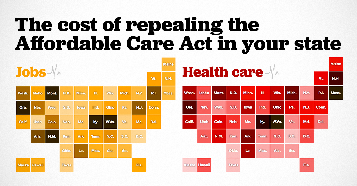
Table 3 shows the states suffering the largest losses as a share of their under-65 population, while the map in Figure A shows, in addition to the net jobs lost, jobs lost as a share of total state employment. The top 15 job-losing states, as measured by jobs lost as a share of both the total employment and the share of residents under age 65, are Arizona, Colorado, Kentucky, Louisiana, Maryland, Montana, Nevada, New Jersey, New Mexico, North Carolina, Oregon, Rhode Island, Vermont, Washington, and West Virginia.
Job losses resulting from ACA repeal as a share of total state employment
| State | Drop in overall state employment | Number of jobs lost |
|---|---|---|
| Washington D.C. | 0.19% | -1,466 |
| South Dakota | 0.19% | -825 |
| Utah | 0.22% | -3,104 |
| Virginia | 0.26% | -10,243 |
| Nebraska | 0.27% | -2,788 |
| Wisconsin | 0.28% | -8,290 |
| Kansas | 0.30% | -4,148 |
| Texas | 0.33% | -40,550 |
| South Carolina | 0.37% | -7,693 |
| Oklahoma | 0.38% | -6,354 |
| Wyoming | 0.42% | -1,168 |
| Iowa | 0.43% | -6,753 |
| Missouri | 0.50% | -14,077 |
| Pennsylvania | 0.53% | -31,387 |
| Minnesota | 0.55% | -15,806 |
| Massachusetts | 0.55% | -19,640 |
| New York | 0.56% | -52,203 |
| North Dakota | 0.56% | -2,460 |
| Maine | 0.56% | -3,435 |
| Georgia | 0.57% | -25,090 |
| Alabama | 0.58% | -11,459 |
| Indiana | 0.59% | -18,111 |
| Hawaii | 0.66% | -4,299 |
| Mississippi | 0.67% | -7,684 |
| New Hampshire | 0.71% | -4,801 |
| Idaho | 0.76% | -5,310 |
| Delaware | 0.76% | -3,497 |
| Florida | 0.76% | -64,629 |
| Connecticut | 0.76% | -12,836 |
| Illinois | 0.78% | -47,060 |
| Arkansas | 0.79% | -9,737 |
| Tennessee | 0.80% | -23,877 |
| Alaska | 0.81% | -2,702 |
| California | 0.85% | -141,676 |
| Michigan | 0.89% | -38,720 |
| Ohio | 0.91% | -50,343 |
| Vermont | 0.95% | -2,991 |
| Maryland | 1.01% | -27,398 |
| North Carolina | 1.12% | -48,925 |
| Nevada | 1.25% | -16,332 |
| Colorado | 1.34% | -35,217 |
| Washington | 1.36% | -44,654 |
| Louisiana | 1.42% | -28,063 |
| New Jersey | 1.51% | -61,544 |
| Arizona | 1.55% | -41,982 |
| Rhode Island | 1.63% | -8,036 |
| West Virginia | 2.00% | -15,412 |
| Montana | 2.27% | -10,599 |
| Oregon | 2.28% | -42,348 |
| Kentucky | 2.92% | -55,949 |
| New Mexico | 3.86% | -31,853 |
Source: Based on data from Table 1 as well as multipliers from Bivens and Fieldhouse (2012) and Chodorow-Reich et al. (2012) and methods outlined in Bivens (2014), as described in the text and the technical appendix
Conclusion
The ACA is primarily health and financial security policy, not a jobs program. But, because the scale of the uninsured problem in the United States was so large pre-ACA and because health care is so expensive and such a significant share of the overall U.S. economy, the ACA’s fiscal provisions are necessarily large. This scale means that its implementation and its potential repeal became de facto macroeconomic policy and thus affects jobs. When the Medicaid expansion and insurance and cost-sharing subsidies were implemented in 2014, they provided a noticeable (and needed) boost to states’ economies and job markets. Even with the fiscal boost provided by the ACA, overall fiscal policy at both the state and federal level was extraordinarily austere in the post-2011 portion of the recent economic recovery, relative to previous economic recoveries. This spending austerity entirely explained the historically slow growth in the recovery after 2011. This austerity would clearly have been even worse without the provisions of the ACA. And repealing the ACA would constitute a contractionary fiscal shock going forward that would reduce the pace of economic growth and cost jobs.
Of course, the primary reason to oppose repeal (let alone build upon the ACA to reach a genuinely universal system of health coverage) is to protect the increased health and financial security that the ACA extended to tens of millions of Americans. But the macroeconomic effect of rapidly unraveling it is significant, and some states will suffer more than others. Policymakers should bear this in mind. Excessive austerity has already prevented a full and timely recovery from the Great Recession. It would be a shame to throttle the pace of recovery further by repealing what could become a key and valued part of the American social insurance system.
About the author
Josh Bivens joined the Economic Policy Institute in 2002 and is currently the director of research. His primary areas of research include macroeconomics, social insurance, and globalization. He has authored or co-authored three books (including The State of Working America, 12th Edition) while working at EPI, edited another, and has written numerous research papers, including for academic journals. He often appears in media outlets to offer economic commentary and has testified several times before the U.S. Congress. He earned his Ph.D. from The New School for Social Research.
Technical appendix
This appendix provides some more explanation of the data and methods used to construct Tables 1 and 3 in the text.
Notes on Table 1
The data on federal spending flows for Medicaid expansions, insurance premium subsidies, and cost-sharing subsidies for each state are taken directly from Blumberg, Buettgens, and Holahan (2016), which also provides an estimate of how much states that expanded Medicaid under the ACA also boosted their own (nonfederal) spending on Medicaid. We have not included these nonfederal spending increases in the spending flows summarized in Table 1. The Blumberg, Buettgens, and Holahan (2016) estimates are projections for 2019.
The data for tax cuts that would flow to each state if ACA were repealed are estimated by combining data from the Tax Policy Center (2016) and Frank (2017). The Tax Policy Center estimates the incidence of tax cuts (i.e., the distribution of tax cuts by tax unit income level) that would be triggered by ACA repeal. The TPC projections are for 2017. To make these congruent with the 2019 spending changes projected by Blumberg, Buettgens, and Holahan (2016), we boost the aggregate amount of tax cuts by 9 percent, based on what the Congressional Budget Office (2016) projected about growth in personal income over the next two years.
As documented in the text, these tax cuts are extraordinarily regressive, with just under 60 percent of the benefits going to the top 1 percent of households. We allocate the incidence of these tax cuts across states simply by distributing them proportionally to each state’s share of the (national) income fifths, supplemented with data on each state’s share of top 1 percent and 10 percent households, in the most recent year for which data is available (2015).
So, for example, California has 15.7 percent of all households that are in the national top 1 percent, so we allocate 15.7 percent of the benefits of the ACA tax cuts that accrue to the national top 1 percent to California. We repeat this for the bottom four-fifths of households as well as for households between the national 80th and 99th percentiles.
State-level shares of the national income fifths are calculated using the ACS. State-level shares of the top 10 percent and top 1 percent of households come from Frank (2017). The national top 1 percent is clearly not spread uniformly across states. States with disproportionately high shares of top 1 percent households that will see disproportionate gains from cutting ACA taxes are New York, California, New Jersey, Massachusetts, Connecticut, Florida, Illinois, Maryland, Virginia, the District of Columbia, and Washington.
Importantly, our method of allocating the tax cuts across states likely understates just how concentrated these benefits are likely to be in those states with higher shares of the top 1 percent. States with high shares of households in the top 1 percent are also likely to have even higher shares of total income earned by the top 1 percent in their state. This can be seen by looking at the share of the (national) 0.1 percent in each state. States that have large shares of the top 1 percent have even higher shares of the top 0.1 percent. Since we know that incomes of the top 0.1 percent constitute half of all income in the top 1 percent, this means that the total income share of the top 1 percent across states is likely even more concentrated than just a simple headcount of the top 1 percent. In short, the states that disproportionately gain from the ACA tax cuts likely will see even larger benefits than our allocation estimates.
Notes on Table 3
For translating the change in tax and spending flows by state into employment outcomes, we first use output multipliers collected by Bivens and Fieldhouse (2012) to translate the changes in taxes and premium and cost-sharing subsidies into changes in output. For premium and cost-sharing subsidies, we apply a multiplier of 1.25, which is essentially the multiplier estimated by various sources for the payroll tax holiday in 2010. Because the incidence of premium and cost-sharing subsidies is actually more progressive than the payroll tax holiday, this is a conservative choice. For the tax changes, we apply the 0.32 multiplier reported by Bivens and Fieldhouse (2012) for the full collection of tax cuts enacted during the presidency of George W. Bush. Again, given that the benefits of repealing all of the 2001 and 2003 Bush tax cuts are less regressive than the repeal of ACA tax cuts, this seems a safe choice.
For translating the Medicaid spending changes into output changes, we apply the output multiplier of 2.1 consistent with output multipliers estimated by Chodorow-Reich et al. (2012). 8 Their estimates have several advantages. First, they are estimated exactly from previous changes in Medicaid spending; the authors estimated the employment effects across states that were spurred by the increase in federal Medicaid spending included in the ARRA. Further, these estimates are extraordinarily high-quality. They are based on a natural experiment that provided a purely exogenous shock to Medicaid spending. This is essentially the gold standard in empirical macroeconomics.
We then translate the estimated output changes into employment changes based on the methods explained in Bivens (2011), and summarized here. Essentially, each 1 percent increase in output is assumed to translate into a 1 percent change in FTE employment on average. As Bivens (2011) points out, a 1 percent change in output often translates into a less than 1 percent change in overall employment as productivity and average hours worked can change and soak up some of the increase or decrease in labor demand spurred by rising or falling output. A large contractionary shock could well result in lower labor demand accommodated in part through fewer average hours worked per week rather than a smaller number of employees. But we can sidestep this problem by estimating the change in FTE employment, holding average hours fixed by definition.
To translate this rule of thumb into jobs per dollars gained in output, we take the ratio of gross domestic product and total full-time equivalent employment in 2015. This ratio implies that each $138,000 of output translated into one (FTE) job in 2015. To make this comparable with the 2019 projections on taxes and spending, we boost this number by 6 percent, to account for projected productivity growth between 2015 and 2019. This yields one job created for every $146,000 in output.
A note about applicable multipliers in today’s economy
It could be argued that the Bivens and Fieldhouse (2012) and Chodorow-Reich et al. (2012) multiplier estimates are not applicable to today’s economy. Both studies examine multipliers measuring the effect of fiscal shocks in an economy in which the Federal Reserve is willing to accommodate fiscal support, i.e., the Fed does not respond to federal spending increases by rate hikes designed to stave off inflation. This lack of any countervailing monetary policy reaction is why the fiscal change yields such large effects (or high multipliers). Today’s unemployment rate is roughly equal to what prevailed before the Great Recession, so many have argued that the U.S. economy is now at full employment, and so the Fed will counteract any large fiscal changes. Further, the full fiscal impact of ACA repeal is commonly expected to only occur in a few years (2019 is commonly cited). In the minds of many, this means that the economy and national labor market will be even tighter (closer to full employment) than it is today. According to this line of thinking, projections of employment losses in 2019 based on large fiscal changes need to account for a large (and importantly, effective) countervailing monetary policy change.
However, we find this reasoning incorrect on a few fronts.
First, there is no compelling evidence that the U.S. economy is clearly pinned at maximum employment. As noted earlier, plenty of labor market indicators—the headline unemployment rate, prime-age employment-to-population ratios, wage growth measures, quits rates—were all much tighter in the late 1990s/2000 labor market. And yet these turn-of-the-century labor markets did not spark accelerating inflation. So, there is plenty of reason to think that the U.S. economy remains demand-constrained relative to its productive capacity and that employment (and perhaps even productivity) could be boosted with faster demand growth. Further, even though the full fiscal impact of ACA repeal is conventionally thought to take place only in 2019, projections by the Federal Reserve do not show a huge amount of labor market tightening between now and then. In fact, today’s unemployment rate is a bit below what the Fed seems to be projecting as the so-called natural rate—the lowest rate of unemployment that is sustainable in the long run without accelerating inflation.9
Second, if what was under discussion was an expansionary fiscal shock, the claim that it would be neutralized by countervailing Federal Reserve policy would be more convincing. In this case, it would not matter whether the economy was actually at full employment, all that would matter was whether the Fed thought the economy was at full employment. As long as they decided the economy was at full employment, they would try to neutralize any expansionary fiscal shock with contractionary monetary policy.
But to avoid any employment losses (even in 2019) stemming from a large fiscal contraction, the Fed would need to be willing and able to neutralize this through responsive and effective expansionary monetary policy. Their ability to do so is highly uncertain. The same Fed projections indicating that today’s unemployment rate is higher than the long-run natural rate also predict that the Fed’s short-term policy rate is likely to be just 2.1 percent going into 2019. This provides the Fed with very little conventional ammunition to neutralize a large contractionary fiscal shock (i.e, with little room to lower interest rates). In the last five recessions, for example, the peak-to-trough change in the federal funds rate as the Fed aimed to stop contraction and spur recovery was over 3.5 percent.
Further, Angrist, Jordà, and Kuersteiner (2013) provide compelling evidence that while the Fed has substantial power to slow recoveries and to neutralize expansionary fiscal shocks with higher interest rates, they have much more limited ability to spur recovery in the face of fiscal contractions with interest rate cuts. They find that a -0.25 percentage-point initial change in the federal funds rate is associated with a 1.5 percentage-point decline in these rates over the next two years but that this cumulative reduction has essentially no significant effect on unemployment.
It could be the case that other, non-ACA elements of the coming economic agenda will provide such a large expansionary fiscal boost to the economy that the ACA repeal will be overwhelmed and no employment loss will be experienced. If, for example, large deficit-financed tax cuts or infrastructure spending plans are passed by Congress and the president, this could provide enough of a fiscal boost to absorb the ACA repeal without large macroeconomic effects. However, the same members of Congress who are calling for large tax cuts are also calling for sharp deficit reduction and steep spending cuts to income-support programs targeted at the lowest-income households. These latter stated priorities would result in a large fiscal drag, not a boost. In short, non-ACA fiscal policy moves are uncertain, and so it makes sense, given how large the tax and spending cuts associated with ACA repeal would be, to assess their macroeconomic effects.
Endnotes
1. The ACA also includes several regulatory changes that are important for health policy reasons but do not have any direct impact on overall employment, which is the primary focus of this report.
2. A recent study by Ku et al. (2017) undertook a similar estimate of potential job losses caused by ACA repeal. Our study uses slightly different estimates of the spending cutbacks that would be caused by ACA repeal and also uses macroeconomic multipliers rather than the regional multipliers used by Ku et al. (2017). The most important difference, however, is that our study also accounts for the fiscal stimulus provided by tax cuts embedded in ACA repeal.
3. The premium and cost-sharing subsidies were administered largely through the tax code, and are sometimes referred to as tax cuts rather than spending increases. Because they are refundable (i.e., they can be claimed in full even by households without income tax liability to support their full value), and because they are not appropriated annually, they share many characteristics with mandatory spending in the form of income transfers (e.g., federal spending in the form of Social Security payments to beneficiaries or unemployment benefits to laid-off workers). For the purposes of this brief, we will refer to them as spending rather than tax credits.
4. Specifically, the TPC analysis is of tax units, but these are close to conventional definitions of households so we feel comfortable melding the two together.
5. Non-expansion states still have some federal Medicaid dollars affected by ACA repeal, however. While some Medicaid expansions required state approval, the ACA mandated that children ages 6–18 in families with incomes between 100 and 138 percent of the federal poverty level be eligible for Medicaid. If this is rolled back with reform and states revert to pre-ACA conditions, at least some of these children will no longer be covered by Medicaid, and the states will lose the matching funds. Further, if ACA repeal eliminates the individual mandate to obtain insurance coverage, Medicaid rolls could shrink, and states would see a corresponding cutback in federal spending flows.
6. We should be clear that never expanding Medicaid means that states have missed out on years of insurance coverage for their most vulnerable citizens as well as the fiscal boost from these spending flows. So, the lighter relative burden of repeal for these states is just the flip side of having rejected any benefits in the past.
7. A 2 percent price inflation target is consistent with roughly 3.5-4 percent nominal wage growth in a healthy economy following a steep recession. For a full reasoning why see Bivens (2014).
8. The Chodorow-Reich et al. (2012) paper actually directly estimates employment gains from Medicaid changes. They find extraordinarily large employment effects (one job created through every $30,000 in Medicaid spending, with three-quarters of this effect coming in private-sector, non–health care related jobs). But they argue that the implied output effects are consistent with studies showing output multipliers a bit over 2. In fact, the implied output effects are also consistent with output multipliers as high as 3, but we take the lower end of the range for this report.
9. Of course, the future is uncertain, and the Congressional Republicans could well decide to put repeal of ACA on a fast-track. Further, even if the plan is to delay full unraveling of the ACA spending provisions until 2019, Blumberg, Buettgens, and Holahan (2016) point out that repeal could near-instantly cause an unraveling of the individual marketplace for insurance. If this unraveling causes people to stop searching for health insurance through the exchanges, this would lead to a large decline in premium and cost-sharing subsidies distributed through these exchanges. This alone could constitute a nontrivial and much more immediate contractionary fiscal shock.
References
American Community Survey (2017). Microdata accessed January 2017.
Angrist, Joshua, Òscar Jordà, and Guido M. Kuersteiner. 2013. “Semiparametric Estimates of Monetary Policy Effects: String Theory Revisited,” Working Paper Series 2013-24, Federal Reserve Bank of San Francisco.
Bivens, Josh. 2011. Method Memo on Estimating Jobs Impact of Various Policy Changes. Economic Policy Institute report.
Bivens, Josh. 2014. Another Vital Indicator for Monetary Policy: Nominal Wage Targets. Report for Policy Futures project. http://www.cbpp.org/research/full-employment/a-vital-dashboard-indicator-for-monetary-policy-nominal-wage-targets
Bivens, Josh and Andrew Fieldhouse. 2012. A Fiscal Obstacle Course, Not a Cliff: Economic Impacts of Expiring Tax Cuts and Impending Spending Cuts, and Policy Recommendations. Economic Policy Institute report.
Blumberg, Linda, Matthew Buettgens, and John Holahan. 2016. Implications of Partial Repeal of the ACA through Reconciliation. Urban Institute Report.
Chodorow-Reich, Gabriel, Laura Feiveson, Zachary Liscow, and William Gui Woolston. 2012. “Does State Fiscal Relief during Recessions Increase Employment? Evidence from the American Recovery and Reinvestment Act.” American Economic Journal: Economic Policy, vol. 4 no. 3, 118–145.
Frank, Mark. 2017. Unpublished estimates available upon request from author, based on data collection stored at: http://www.shsu.edu/~eco_mwf/inequality.html
Ku, Leighton, Erika Steinmetz, Erin Brantley, and Brian Bruen. 2017. The Economic and Employment Consequence of Repealing Federal Health Reform: a 50 State Analysis. Milken Institute School of Public Health, Department of Health Policy and Management, George Washington University.
Tax Policy Center. 2016. Tables from: http://www.taxpolicycenter.org/simulations/distribution-affordable-care-act-taxes-dec-2016
U.S. Census Bureau (2016). Microdata from March 2016 Current Population Survey (Annual Social and Economic Supplement).