Briefing Paper #374
Executive summary
In U.S. policymaking circles in recent years there have been recurrent calls to increase infrastructure investments. This is hardly a surprise, as increased infrastructure investments could go a long way to solving several pressing challenges that the American economy faces.
In the near term, the most pressing economic challenge for the U.S. economy remains the depressed labor market. As of May 2014, the share of prime-age adults (age 25–54) currently employed is just 0.5 percentage points higher than it was at the official end of the Great Recession in June 2009. And it is more than 3.9 percentage points lower than during the labor market peak of the mid-2000s, and 5.4 percentage points lower than its 1999 peak.
In the longer term, the most pressing economic challenges for the U.S. economy concern how to provide satisfactory living standards growth for the vast majority of people. Such growth requires two components: rapid overall productivity growth, and a stabilization (or even reversal) of the large rise in income inequality that occurred in the three decades before the Great Recession, a rise in inequality that kept overall productivity growth from translating into living standards growth for most Americans.
This report examines the short- and long-term economic and employment impacts of infrastructure investment. It examines three possible scenarios for infrastructure investment and estimates their likely impact on overall economic activity, productivity, and the number and types of jobs, depending on how the investments are financed. The data show that by far the biggest near-term boost to gross domestic product and jobs comes from financing the new investment through new federal government debt rather than a progressive increase in taxation, a regressive increase in taxation, or cuts to government transfer programs. Our research also shows that this debt-financed impact is greater than that deriving from increases in infrastructure investment that are driven not by direct public investments but through other actions, such as regulatory mandates.
Key findings of the report are:
Three potential infrastructure packages would yield from $18 billion to $250 billion annually for infrastructure investment.
- Scenario one cancels all of the scheduled cuts stemming from the budget “sequester” (automatic, across-the-board cuts to discretionary spending called for in the Budget Control Act (BCA) of 2011), yielding an average of $30 billion annually over the next decade for infrastructure investments. (As of January 2014, a third of the scheduled sequester cuts were cancelled for the next two years only.)
- Scenario two implements a package of green investments that includes a large increase in investments in the energy efficiency of residential and commercial buildings and upfront investments to construct a national “smart grid,” yielding $92 billion annually in infrastructure investments over the next decade.
- Scenario three makes an ambitious investment in largely traditional infrastructure projects in transportation and utilities (particularly water treatment, distribution, and sewage systems) to nearly close the U.S. “infrastructure deficit” identified by the American Society of Civil Engineers (ASCE) and yield $250 billion annually in infrastructure investment between now and 2020.
In the near term, increases in infrastructure spending would significantly boost economic activity and employment.
- Under scenario one, a debt-financed $18 billion annual investment in infrastructure yields a $29 billion increase in GDP and 216,000 net new jobs by the end of the first year, with the increased levels then sustained over the next decade.
- Under scenario two, a debt-financed package of green investments totaling $92 billion annually boosts GDP by $147 billion and generates 1.1 million net new jobs by the end of the first year, with the increased levels then sustained over the next decade.
- Under scenario three, a debt-financed $250 billion annual investment boosts GDP by $400 billion and overall employment by 3 million net new jobs by the end of the first year, with the increased levels then sustained over the seven-year life of the investment.
- Any method of making these infrastructure investments deficit-neutral reduces their impact on near-term activity and employment, but every method except cuts to government transfers still leaves a net positive impact.
Over the long term, we can reliably predict only the impact of infrastructure investments on the composition, not the overall level, of labor demand.
Because the impact of infrastructure investments on the overall level of economic activity depends on the degree of productive slack in the economy, the stance of monetary policy, and how the investments are financed, it is impossible to reliably forecast the long-term (further than five years out) effects of such investments on the overall level of economic activity. However, we can reliably project the impact of infrastructure investments on the composition of labor demand. Even if these investments crowd out other forms of spending and do not affect the overall level of activity and employment, it remains the case that composition of employment supported by additional spending on infrastructure would be different than that of the economic activity it potentially displaces.
- Under all scenarios, jobs created are disproportionately male, Latino, and skewed away from younger workers.
- Under scenario one, male employment accounts for 77 percent of all jobs created, while under scenario two it accounts for 80.4 percent of all jobs created, and under scenario three it accounts for 74.1 percent, compared with an economy-wide average of 50.2 percent of all jobs being held by men.
- Under scenario one Latino employment accounts for 15.4 percent of all jobs created, while under scenario two it accounts for 16.2 percent of all jobs created, and under scenario three it accounts for 14.3 percent, compared with an economy-wide average of 12.3 percent.
- Under scenario one, employment of young adults (under 25 years old) accounts for 9.3 percent of all jobs created, while under scenario two it accounts for 9.5 percent of all jobs created, and under scenario three it accounts for 7.8 percent, compared with an economy-wide average of 13.2 percent.
- Under all scenarios, jobs created are disproportionately filled by workers without a four-year university degree. Under scenario one, workers with a bachelor’s degree or more education fill 23 percent of all jobs created, while under scenario two college-educated employment accounts for 19.6 percent of all jobs created, and under scenario three it accounts for 21.4 percent, compared with an economy-wide average of 32.6 percent.
- Under all scenarios, jobs created are disproportionately middle- and/or high-wage. Under scenario one employment in the bottom wage quintile accounts for just 9.5 percent of all jobs created, while under scenario two it accounts for 9.4 percent of all jobs created, and under scenario three it accounts for 11.2 percent of all jobs created, compared with an economy-wide average of 18.9 percent.
Infrastructure investments provide the potential to boost economy-wide productivity growth.
Productivity growth has slowed significantly in the U.S. economy, beginning even before the onset of the Great Recession. Our analysis conforms with a large and growing body of research persuasively arguing that infrastructure investments can boost even private-sector productivity growth.
- An ambitious effort to increase infrastructure investment by $250 billion annually over seven years would likely increase productivity growth by 0.3 percent annually—a boost more than half as large as the productivity acceleration in the U.S. economy between 1995 and 2005, one that was attributed to information and communications technology (ICT) advances.
- A productivity acceleration of 0.3 percent would have measurable impacts on the estimated Non-Accelerating Inflation Rate of Unemployment (NAIRU) and could allow macroeconomic policymakers to target significantly lower rates of unemployment. Extrapolating from the experience of the late 1990s, the NAIRU could be lowered by as much as 1 full percentage point by a sustained $250 billion annual increase in infrastructure investment. This could mean that more than 1 million additional workers each year find employment.
List of acronyms used in this report
ASCE = American Society of Civil Engineers
GDP = gross domestic product
BCA = Budget Control Act
ICT = information and communications technology
NAIRU = non-accelerating inflation rate of unemployment
GCC = global climate change
GHG = greenhouse gases
EPRI = Electric Power Research Institute
PPM = parts per million
CPC = Congressional Progressive Caucus
NIPA = National Income and Product Accounts
BEA = Bureau of Economic Analysis
OMB = Office of Management and Budget
EPI = Economic Policy Institute
ERM = Employment Requirements Matrix
BLS = Bureau of Labor Statistics
ARRA = American Recovery and Reinvestment Act
PERI = Political Economy Research Institute
CPS = Current Population Survey
CBO = Congressional Budget Office
CEA = Council of Economic Advisers
MAEC = Moody’s Analytics’ Economy.com
CPS-ORG = Current Population Survey Outgoing Rotation Group
QCEW = Quarterly Census of Employment and Wages
U.S. = United States
MPC = marginal propensity to consume
ZLB = zero lower bound
VAR = vector auto-regression
HELP = health, education, leisure, hospitality, business and professional services
Scenarios for infrastructure investments
Simple political realism about the current state-of-play of American fiscal policy argues that large-scale infrastructure investments financed by the federal government are unlikely in coming years. However, economic analysis stands apart from current politics, and the economic case for boosting these investments is strong—and perhaps made even stronger by the growing threat of global climate change (GCC) caused by greenhouse gas (GHG) emissions.
Given these conflicting imperatives—political realism versus economic necessity—this report examines three different scenarios for infrastructure investments. The first looks at the implications for infrastructure investment if sharp cuts to federal discretionary spending called for in the Budget Control Act of 2011 are cancelled.1 A 2013 budget deal signed into law does indeed cancel a portion (but just a portion) of the automatic sequester cuts for the next two years. Given this, the paper examines what reversing these cuts completely would mean for boosting future infrastructure investments.
The second scenario is more ambitious, and addresses the need for the United States to transition to an economy that emits fewer greenhouse gases. It packages a mix of investments in energy efficiency in the building sector with start-up investments in a national “smart grid.” The dollar figure for building efficiency investments is taken from a (now-famous) McKinsey report detailing the benefits of energy efficiency. For this scenario, we identify all building efficiency investments that were identified by McKinsey as having a net negative cost over the useful lives of the projects. For the smart-grid investments, we relied on assessments from the Electric Power Research Institute (EPRI) for the upfront costs. After estimating these two components of this “green” package of energy, we checked to ensure that it would constitute a genuinely ambitious step toward mitigating GHG emissions, using work by Pacala and Socolow (2004).
Pacala and Socolow (2004) introduced the concept of the “stabilization wedge” of GHG abatement. They essentially look at the decline in carbon emissions needed to stabilize atmospheric concentrations of carbon at 450 parts per million (PPM) by 2054, a benchmark that they identify as the minimally ambitious goal for reducing the future costs imposed by climate change.2
They next divided the entire wedge between carbon emissions projected to occur under a “business as usual” (BAU) scenario and the emissions that would be allowed under a scenario that kept carbon at less than 450 parts per million into seven smaller “sub-wedges”. Next they identified a number of actions that would be sufficient to “fill” one of these smaller sub-wedges. So, for example, increasing fuel efficiency of 2 billion cars from 30 mpg to 60 mpg would constitute one sub-wedge, while boosting coal-fired power plant efficiency by 50 percent would constitute another sub-wedge.
The package of green investments that constitutes our second infrastructure investment scenario would seem to be ambitious indeed—probably coming close to accounting for well over half of a stabilization sub-wedge, meaning that this package would be moving the U.S. economy more than 10 percent of the way toward stabilizing GHG emissions at 450 PPM by itself.
The building investments alone likely account for well over half of a stabilization wedge. Pacala and Socolow (2004) identify “cut[ing] carbon emissions by one-fourth in buildings and appliances” as a wedge. The McKinsey report estimates that the efficiency investments called for in it would lead to almost exactly a one-quarter reduction in carbon emissions (23 percent), with more than 60 percent of this efficiency effect coming from the buildings channel alone.
Further, EPRI has identified a number of ways a smart grid could facilitate the achievement of other stabilization wedges. For example, they note that a smart grid could accommodate an increase in electric and hybrid automobiles, which could help achieve the stabilization wedge possible through increased fuel efficiency of cars. And they note that household efficiencies would be much easier to achieve if energy savings stemming from them were more salient to households, and that this salience would be much easier to achieve through “smart metering” and other mechanisms that more closely tie household energy bills to their consumption patterns.
The last scenario examines an across-the-board increase in infrastructure spending concentrated in traditional transportation and utilities investments. The magnitude of this spending—$250 billion annually—is chosen to close the “infrastructure deficit” identified by the American Society of Civil Engineers (ASCE) in recent reports about the state of the nation’s infrastructure, including its most recent such report (ASCE 2013).
Scenario One: Undoing the discretionary spending caps imposed by the 2011 Budget Control Act
In 2011, the U.S. Congress passed the Budget Control Act (BCA), which significantly reduced 10-year discretionary spending growth. Most of the American social insurance system (Social Security, Medicare, Medicaid, and the Affordable Care Act) was unaffected. However, because the vast bulk of public investments (including infrastructure investments) are financed by the discretionary side of the federal budget, these spending caps—including the now-famous budget “sequester”—have steep consequences for infrastructure spending. Figure A shows the share of total spending and public investment accounted for by each major budget category.
The bars on the left of each two-bar set show the share of total federal spending accounted for by each of the three major spending categories. Nondefense discretionary spending accounts for 21.0 percent of total federal spending, defense spending accounts for 20.4 percent, while mandatory spending (dominated by the retirement security programs Medicare and Social Security as well as other health spending) accounts for 58.7 percent.
The bars on the right of each two-bar set show the share of total federal public investment accounted for by each of the three major spending categories. Nondefense discretionary spending, despite accounting for just a fifth of total spending, accounts for well over half of total public investment, 55.4 percent. Defense spending accounts for 39.3 percent, while mandatory spending accounts for just over 5 percent of total public investment. What this figure demonstrates is that any policy change that leads to large changes in the trajectory of discretionary spending will almost inevitably have large impacts on the future course of public investment.
Average share of total U.S. federal spending and total federal public investment, by major budget category, 2010–2012
| Federal spending | Federal public investment | |
|---|---|---|
| Nondefense discretionary | 21.0% | 55.4% |
| Defense | 20.4% | 39.3% |
| Mandatory | 58.7% | 5.3% |
Source: Author's analysis of unpublished data from the Office of Management and Budget (OMB)
In estimating the impacts on economic activity and employment from undoing these spending caps, we assume that the composition of discretionary spending is essentially unchanged by shifts in the level of spending. It is theoretically true that cuts to infrastructure spending could be less or more steep than overall spending cuts, but this is nearly impossible to forecast. Further, the discretionary spending cuts currently constituting the policy baseline in the United States (i.e., the budget “sequester”) are across-the-board cuts to every category of discretionary spending, making the assumption that the composition of discretionary spending cuts will be unaffected by the level in fact consistent with current budget law.
While economic analysis of the nation’s infrastructure needs would drive public investment policy in a more rational world, it is important to emphasize what an uphill struggle it will be in coming years to overcome the political barriers to increasing public investment. Figure B shows the implications for overall public investment if various 2014 budget proposals were passed. The budget proposals include, on the Democratic side, those from the White House (the Obama plan), the Senate Budget Committee (Murray plan), Democrats in the House of Representatives (House Democratic budget alternative), and the Congressional Progressive Caucus, and, on the Republican side, that of the House Committee on the Budget (Ryan plan). It demonstrates clearly the downward pressure of austerity on public investment possibilities, with nearly all budget proposals coming from the U.S. Congress, except the Congressional Progressive Caucus (CPC) budget, calling for steep cuts in coming years. (See the text box titled “U.S. budget politics” for a broad overview of the differences between the budgets and an explanation of why there are so many competing budget proposals in U.S. politics today.) On the one hand, these projections show the widespread acceptance of large cuts in discretionary investment (and hence public investment) in coming years, which just highlights the political hurdles to increased infrastructure spending. On the other hand, these scenarios show just how much room there is in coming years to boost infrastructure spending just by returning the public commitment to it to recent historic norms.
Actual and implied public investment as a share of GDP under various 2013 U.S. budget proposals, 2000–2023
| House Democratic budget alternative | Ryan plan (House) | Murray plan (Senate) | Congressional Progressive Caucus | Obama plan (White House) | |
|---|---|---|---|---|---|
| 2000 | 3.2% | ||||
| 2001 | 3.1% | ||||
| 2002 | 3.2% | ||||
| 2003 | 3.2% | ||||
| 2004 | 3.1% | ||||
| 2005 | 3.1% | ||||
| 2006 | 3.2% | ||||
| 2007 | 3.3% | ||||
| 2008 | 3.4% | ||||
| 2009 | 3.4% | ||||
| 2010 | 3.3% | ||||
| 2011 | 3.0% | 3.0% | 3.0% | 3.0% | 3.0% |
| 2012 | 3.2% | 3.1% | 3.1% | 3.2% | 3.1% |
| 2013 | 3.4% | 3.2% | 3.2% | 3.4% | 3.3% |
| 2014 | 3.3% | 3.0% | 3.2% | 3.5% | 3.1% |
| 2015 | 3.1% | 2.8% | 3.1% | 3.5% | 3.0% |
| 2016 | 2.9% | 2.7% | 2.9% | 3.4% | 2.9% |
| 2017 | 2.8% | 2.6% | 2.8% | 3.2% | 2.8% |
| 2018 | 2.7% | 2.5% | 2.7% | 3.1% | 2.7% |
| 2019 | 2.7% | 2.5% | 2.6% | 3.1% | 2.7% |
| 2020 | 2.6% | 2.4% | 2.6% | 3.0% | 2.6% |
| 2021 | 2.6% | 2.4% | 2.5% | 3.0% | 2.6% |
| 2022 | 2.5% | 2.3% | 2.5% | 2.9% | 2.5% |
| 2023 | 2.5% | 2.3% | 2.4% | 2.9% | 2.4% |

Source: Author's analysis based on Bivens (2013)
U.S. budget politics
The normal federal budget process in the United States essentially disintegrated between 2010 and 2013. Because Republicans controlled the House of Representatives while Democrats controlled the Senate, no agreement could be reached on annual budgets. Instead, government spending levels were set with “continuing resolutions”—extensions of levels dictated by the Budget Control Act (BCA) of 2011, legislation passed to resolve the debt ceiling crisis of the summer of 2011. The BCA mandated steep cuts in domestic discretionary spending, spending that must be appropriated each year and which largely excludes the expensive social insurance programs such as Social Security, Medicare, Medicaid, and the newly passed Affordable Care Act.
This failure to agree on annual budgets also led to a proliferation of competing budget proposals. By custom, the budget committees of both the House of Representatives and the Senate are charged with submitting budget proposals, as is the president. Again, because the House budget committee was run by Republicans while the Senate budget committee was run by Democrats, there were large differences between the respective budget committee proposals (shorthanded by the names of their respective chairs, with the Republican House plan known as the “Ryan plan” after Rep. Paul Ryan (R-Wis.), and the Democratic Senate plan as the “Murray plan” after Sen. Patty Murray (D-Wash.)). The White House budget proposal (shorthanded as the “Obama plan” after President Barack Obama) was very close to the Murray plan.
Besides these proposals, in recent years a number of caucuses within the House and Senate also have been putting forward alternative budget plans. The most ambitious of these were the budget proposals forwarded by the Congressional Progressive Caucus (or CPC). The CPC budgets allowed for much larger deficits in the early years of the budget window to finance infrastructure and other public investment programs aimed at spurring a full recovery from the Great Recession. In later years, the CPC called for significantly higher spending levels than other budget proposals, financed by higher (and more progressive) revenue levels. Figure B in the main body of this report distills the key differences relevant to the analysis in this report—the large differences among various budgets in nondefense discretionary spending levels (the portion of the budget that generally finances the large majority of infrastructure spending).
Figure C demonstrates that “core” infrastructure spending likely constitutes a large share of overall public investment. The Figure examines the portion of public investment classified as structures and does not cover equipment, as only data on structures are broken down in detail that allows us to differentiate core infrastructure investment from other forms of public investment. What the figure shows is that most of what is classified as public investment in official data sources on public investment in structures is indeed infrastructure spending (highways, transportation projects, water and sewer projects, utilities, etc.).
"Core" infrastructure investment and health and education investment in the United States, as a share of GDP, 1947–2011
| Core infrastructure | Health and education | |
|---|---|---|
| 1947 | 0.86% | 0.12% |
| 1948 | 1.00% | 0.30% |
| 1949 | 1.38% | 0.52% |
| 1950 | 1.29% | 0.54% |
| 1951 | 1.21% | 0.59% |
| 1952 | 1.23% | 0.59% |
| 1953 | 1.29% | 0.55% |
| 1954 | 1.45% | 0.63% |
| 1955 | 1.37% | 0.65% |
| 1956 | 1.49% | 0.64% |
| 1957 | 1.58% | 0.67% |
| 1958 | 1.69% | 0.71% |
| 1959 | 1.66% | 0.61% |
| 1960 | 1.54% | 0.61% |
| 1961 | 1.62% | 0.62% |
| 1962 | 1.66% | 0.58% |
| 1963 | 1.72% | 0.63% |
| 1964 | 1.70% | 0.65% |
| 1965 | 1.68% | 0.67% |
| 1966 | 1.65% | 0.74% |
| 1967 | 1.56% | 0.78% |
| 1968 | 1.58% | 0.73% |
| 1969 | 1.38% | 0.68% |
| 1970 | 1.40% | 0.62% |
| 1971 | 1.38% | 0.57% |
| 1972 | 1.27% | 0.54% |
| 1973 | 1.19% | 0.55% |
| 1974 | 1.31% | 0.57% |
| 1975 | 1.35% | 0.56% |
| 1976 | 1.20% | 0.49% |
| 1977 | 1.08% | 0.39% |
| 1978 | 1.12% | 0.36% |
| 1979 | 1.17% | 0.36% |
| 1980 | 1.21% | 0.37% |
| 1981 | 1.05% | 0.31% |
| 1982 | 0.96% | 0.29% |
| 1983 | 0.88% | 0.25% |
| 1984 | 0.92% | 0.25% |
| 1985 | 0.93% | 0.27% |
| 1986 | 0.95% | 0.29% |
| 1987 | 0.98% | 0.28% |
| 1988 | 0.95% | 0.30% |
| 1989 | 0.88% | 0.32% |
| 1990 | 0.91% | 0.33% |
| 1991 | 0.89% | 0.37% |
| 1992 | 0.85% | 0.38% |
| 1993 | 0.81% | 0.34% |
| 1994 | 0.80% | 0.34% |
| 1995 | 0.77% | 0.40% |
| 1996 | 0.78% | 0.41% |
| 1997 | 0.78% | 0.45% |
| 1998 | 0.73% | 0.44% |
| 1999 | 0.70% | 0.42% |
| 2000 | 0.72% | 0.46% |
| 2001 | 0.74% | 0.49% |
| 2002 | 0.79% | 0.52% |
| 2003 | 0.78% | 0.54% |
| 2004 | 0.73% | 0.53% |
| 2005 | 0.72% | 0.52% |
| 2006 | 0.73% | 0.52% |
| 2007 | 0.83% | 0.55% |
| 2008 | 0.82% | 0.59% |
| 2009 | 0.90% | 0.64% |
| 2010 | 0.87% | 0.62% |
| 2011 | 0.85% | 0.52% |
Note: "Core" infrastructure investment includes highway, transportation, sewer, and water-treatment investments.
Source: Author's analysis of Bureau of Economic Analysis National Income and Product Accounts (Tables 1.1.5, 5.8.5a, and 5.8.5b)
A similar breakdown between core infrastructure and other public investments for the equipment component of public investments is not available. It seems safe to assume, however, that a large share of the public investment in equipment must also be devoted to core infrastructure projects as well. Airports, water treatment plants, and rail systems, for example, have investment needs that go far beyond the buildings sitting on them.
The message is clear: Unless the proposed cuts in discretionary spending in coming years are done with surgical precision to avoid cutting infrastructure investments, they will deeply impact annual investments. And it should be noted that the budget “sequester” explicitly disallows such discrimination among different discretionary spending priorities and demands across-the-board cuts.
Economic and employment impact
In order to assess the economic and employment impact of the extra infrastructure investment made possible by undoing the BCA spending caps, we need to know just what kinds of infrastructure investments are currently financed by the federal government.
First, we translate proposed cuts in discretionary spending into cuts in overall public investments, using the same data sources we used to construct Figure A (data sources which show the share of each type of federal government spending that is public investment instead of public consumption). These data (available upon request) are non-public data supplied by the Office of Management and Budget (OMB) to EPI. The main contribution of the data is to identify how many dollars in each detailed budget function (of which there are over 6,000) are dedicated to investment, as opposed to current consumption.
Using these data we can estimate the share of these cuts to public investment that will take the form of cuts to infrastructure spending specifically. We do this by using data from the National Income and Product Accounts (NIPA) from the Bureau of Economic Analysis (BEA) to allocate the cuts to infrastructure spending (simply based on our definition that infrastructure investments cover highway, transportation, sewer and water-treatment industries) to the various industries in our input-output model. Table 1 presents these allocations as gains: how much additional infrastructure spending could flow into each of these industries if these proposed cuts were reversed. Overall it shows that a reversal of the proposed cuts would yield an average of $18 billion annually over the next decade for infrastructure investments.
Annual industry spending (model inputs) under scenario one
| $ billions | Share of total | |
|---|---|---|
| Construction (ERM Sector 15) | 9 | 28.9% |
| HVAC equipment (ERM Sector 67) | 1 | 3.3% |
| Engine, turbine, power transmission equipment (ERM Sector 69) | 1 | 3.3% |
| Computer and peripheral equipment (ERM Sector 71) | 1 | 3.3% |
| Communications equipment (ERM Sector 72) | 1 | 3.3% |
| Audio and video equipment (ERM Sector 73) | 1 | 3.3% |
| Electric lighting equipment (ERM Sector 77) | 1 | 3.3% |
| Other electrical equipment (ERM Sector 80) | 1 | 3.3% |
| Motor vehicle manufacturing (ERM Sector 81) | 2 | 7.2% |
| Total | 18 | 100.0% |
Note: Overall total may not sum due to rounding. Annual gains would take place over the next decade.
Source: Author's analysis of Bureau of Labor Statistics Employment Requirements Matrix and analysis of infrastructure investments made possible through ending budget "sequester" of the Budget Control Act of 2011
Unsurprisingly, the cuts—and thus gains—are heavily concentrated in the construction sector, as federally financed infrastructure projects are heavily concentrated in road building and other forms of transit construction. Federally financed infrastructure projects also lean heavily toward the manufacturing sector, with transportation equipment (aerospace, ships and boats, and motor vehicles manufacturing) dominating. The high shares of aerospace and ship building could be driven in part by the fact that defense spending accounts for a non-trivial share of total public investment. As defense spending is also cut by the provisions of the BCA, one could in theory include these in our overall measures. However, for the purposes of this examination we exclude the aerospace and ship-building sectors, as they are probably less associated with traditional infrastructure projects.
Scenario Two: Combining investments in building energy efficiency and the smart grid for carbon mitigation
A second, more ambitious policy proposal combines large increases in infrastructure spending to improve the energy efficiency of buildings, along with start-up investments for a national “smart grid.” The impetus for examining this scenario is to emphasize that the cost of out-of-date infrastructure is likely rising fast given the enormous threat posed by global climate change driven by greenhouse gas emissions.
Building efficiency
For example, a key part of American infrastructure is simply buildings—both residential and commercial, private and publicly owned. We now know that inefficiency of buildings is a huge contributor to excess carbon emissions, and that investments in energy-efficient buildings represent an enormous low-cost opportunity to reduce GHG emissions. While publicly owned buildings are the obvious first place to start an infrastructure investment effort, it should be noted that the economics of GHG emissions imply that a substantial public investment even in boosting efficiency of privately owned buildings would yield high economic returns. Without externalities, inefficient buildings represent a cost only to their owners, and the case for including improvements to these inefficient buildings in an infrastructure effort is weak. But with unpriced externalities, inefficient buildings—even those privately owned—inflict a cost on everybody, and the case for using public resources to improve them is much stronger.
McKinsey and Company (2009) have famously identified more than $500 billion in energy efficiency opportunities that would have negative net economic cost and offer present-value returns of nearly 100 percent over their useful lives. Pacala and Socolow (2004) have identified improving energy efficiency of buildings as a large enough opportunity to by itself account for more than 10 percent of the total possibility for moving carbon emissions to an economically sustainable level. Rogers (2007) has noted that many market failures even besides the unpriced externality of GHG emissions exist in markets for energy efficiency investments, and that these market failures argue for a key public role in fostering this investment. All of this argues strongly that investing in energy efficiency of buildings would be an extraordinarily high-return activity.
Smart-grid investments
Utilities, particularly energy-providing utilities, are part of the classic definition of infrastructure. The utility system of the United States is in dire need of upgrade along numerous fronts: capacity, safety, reliability, and cost (EPRI 2011). Further, the need to foster a smooth transition to an economy where production is less carbon-intensive in the future will require a much different, and much better, national system of electrical power generation. For example, the benefits of putting a price on carbon emissions will only come to pass if electricity consumers reliably see a price signal from changes in electricity use. Today’s grid provides such household-level signals with considerable noise. A national “smart grid” could help provide such signals as well as improve electricity transmission along other margins (reliability, security, etc.).
The Electric Power Research Institute (EPRI 2011) has undertaken a rigorous estimate of the costs and benefits of investing in a state-of-the-art smart grid for the United States. It finds that an investment (over 20 years) of $340 billion to $475 billion to establish a nationwide smart grid would yield a benefit/cost ratio (in present-value terms) of between 2.8 to 6.0. Part of this benefit includes the enabling role that a smart grid would play in implementing some of the stabilization “wedges” identified by Pacala and Socolow (2004). For example, EPRI demonstrates that a key benefit of a state-of-the-art smart grid would be the capacity to provide charging stations for electrical vehicles. The switch from carbon-fuel-based vehicles to electric vehicles accounts for a stabilization wedge by itself in the Pacala and Socolow analysis.
The portfolio of infrastructure investments packaged in this second scenario is obviously politically ambitious for the present moment in the United States. However, it does serve as a useful reminder that potentially high-return investments are numerous, in large part because of the relative decline in public investment in recent decades (a decline reversed for a few years by the American Recovery and Reinvestment Act (ARRA)). Further, the economic returns to “green” investments in particular are likely rising quickly, as the costs of global climate change begin to manifest, and while policy initiatives aiming to put a price on GHG emissions have so far failed. A key benefit of pricing GHG emissions is to make investments in their mitigation profitable, and hence likely to be undertaken by private actors. But the failure to put a price on these emissions in the United States does not have to mean that no action is taken on this front. Instead, public investments, including infrastructure investments, can be begun even before price signals to drive private investments begin.
Model inputs for scenario two
The model inputs for investments in the smart grid were helped greatly by two previous reports. The first, a 2011 report by the Electric Power Research Institute (EPRI), provided the overall cost, as well as providing a breakdown of this cost between transmission and distribution. Further, a report by Pollin, Heintz, and Garrett-Peltier (2009) for the Political Economy Research Institute (PERI) provides an estimate of the industrial inputs needed for investments to update the smart grid. We use the EPRI (2011) number for overall investment effort needed along with the PERI data on the allocation of investment flows into the industries in our model. This package of green investments—a large increase in efficiency investments in the residential and commercial building sectors, along with upfront investments to construct a national smart grid—would lead to $92 billion annually in infrastructure investments over the next decade. In the case of the smart grid, the industrial allocation of these investments is described in Table 2.
Annual industry spending (model inputs) under scenario two
| $ billions | Share of total | |
|---|---|---|
| Energy efficiency | ||
| Construction (ERM 15) | 52 | 56.5% |
| Smart grid | 40 | 43.5% |
| Construction (ERM 15) | 10 | 10.9% |
| Industrial machinery (ERM 68) | 10 | 10.9% |
| Electronic equipment (ERM 79) | 10 | 10.9% |
| Electrical power goods (ERM 12) | 5 | 5.4% |
| Engine, turbine, power transmission equipment (ERM 69) | 5 | 5.4% |
| Subtotal | 40 | 43.5% |
| Total | 92 | 100% |
Note: Annual gains shown would take place over the next decade.
Source: Author's analysis of Bureau of Labor Statistics Employment Requirements Matrix; EPRI (2011); and Pollin, Heintz, and Garrett-Peltier (2009)
Again, given the emphasis on improving the efficiency of buildings, this package of infrastructure spending predictably leans heavily toward construction. However, there are also direct inflows into a number of manufacturing and utility industries.
Scenario Three: An ambitious across-the-board increase in infrastructure spending
Our last scenario looks at a truly ambitious across-the-board increase in infrastructure spending, on a scale sufficient, for example, to close the accumulated “infrastructure deficit” identified by experts such as the American Society of Civil Engineers (ASCE). This scenario was recommended, for example, by the Congressional Progressive Caucus (CPC) in its budget proposals in recent years.
ASCE issues an annual “report card” on the nation’s infrastructure, and in recent years it has given the U.S. investment effort a failing grade (ASCE 2013). It identifies the needed investment to erase the nation’s substantial “infrastructure deficit” between now and 2020 as $3.6 trillion. Further, it estimates that only about half of this investment amount is likely to be provided under the current trajectory of public investment. Given this, for our third scenario we target $250 billion in new infrastructure spending per year until 2020, an amount that would close the remaining half of the needed investments over that time.
Because transportation systems, water distribution, water treatment, and sewage systems figure prominently in the ASCE report’s documentation of the nation’s infrastructure deficit, we allocate roughly three-quarters of the entire $250 billion additional investments to these sectors (which includes construction activities). The remainder is allocated to other utility sectors and to industries associated with efforts needed to expand high-speed Internet access throughout the country.
Model inputs for Scenario Three
The specific receiving industries for infrastructure spending under the third scenario were picked to correspond with these priorities. Table 3 shows the receiving industries, identified by BLS industry code.
Annual industry spending (model inputs) under scenario three
| $ billions | Share of total | |
|---|---|---|
| Electric power generation, transmission, and distribution (ERM 12) | 16 | 6.5% |
| Natural gas distribution (ERM 13) | 16 | 6.5% |
| Water, sewage, and other systems (ERM 14) | 50 | 20.0% |
| Construction (ERM 15) | 83 | 33.0% |
| HVAC and commercial refrigeration manufacturing (ERM 67) | 10 | 4.0% |
| Communications equipment manufacturing (ERM 72) | 10 | 4.0% |
| Semiconductor and other electronic component manufacturing (ERM 74) | 10 | 4.0% |
| Railroad rolling stock manufacturing (ERM 85) | 10 | 4.0% |
| Other transportation equipment manufacturing (ERM 87) | 10 | 4.0% |
| Transit and ground passenger transportation (ERM 99) | 35 | 14.0% |
| Total | 250 | 100.0% |
Note: Annual gains shown would take place between 2014 and 2020.
Source: Author's analysis of Bureau of Labor Statistics Employment Requirements Matrix and ASCE (2013)
Near-term effects of infrastructure spending
In terms of projecting the near-term, net employment impacts of increased infrastructure spending under the scenarios presented in the previous sections, a number of pieces of economic context must be specified. First, how much economic slack exists—particularly in labor markets. Second, and related but not identical to the question of economic slack, how will monetary policy authorities likely respond to a macroeconomically significant increase in infrastructure investments? Third, how will the infrastructure investments be financed? Through public debt? Through increased revenues or user fees? Or through private borrowing or retained earnings?
In the case of near-term increases in infrastructure investments in the U.S. economy, the answers to the first two of these questions are unfortunately quite simple: There is a very large amount of overall economic slack in the U.S. economy today, and monetary policymakers are highly unlikely to try to neutralize demand increases stemming from near-term infrastructure investments. These answers simply reflect that the United States is very far from having fully recovered from the Great Recession of 2008–2009. Figure D shows the amount of slack in two ways, the ratio of actual to potential gross domestic product (GDP) and the share of prime-age adults (25–54) who are employed.3 During the Great Recession (shaded in grey), both of these measures declined precipitously. Since the official end of the Great Recession, in contrast, the reversal has been quite slow—and over the past year steady progress in improving each has nearly stopped completely. This argues strongly that the U.S. economy has large amounts of productive slack.
Two measures of economic slack: Ratio of actual to potential GDP, and employment-to-population ratio (EPOP) for workers age 25–54, 2000–2013

Note: Shaded areas denote recessions.
Source: Author's analysis of Bureau of Economic Analysis National Income and Product Accounts (Table 1.1.6), Congressional Budget Office (2012), and Current Population Survey (CPS) public data series
Further, the Federal Reserve has continually committed to keeping monetary policy extraordinarily accommodative in coming years and has indeed noted that increased fiscal stimulus (like an increase in infrastructure spending) would be useful for macroeconomic stabilization (see, for example, Yellen (2013).
Given this degree of economic slack and promise of monetary policy accommodation, it seems that the most natural assumption for how a near-term increase in infrastructure investments would be financed is simply through new federal government debt. This would allow the investments to have the largest impact on near-term economic activity and employment.
However, we also calculate near-term impacts stemming from infrastructure investments that are financed by a progressive increase in taxation, a regressive increase in taxation, and cuts to government transfer programs. Lastly, we discuss the likely macroeconomic impact of increases in infrastructure investment that are driven not by direct public investments, but through other actions, such as regulatory mandates.
It should be noted that most of the analysis in this section will rely on a set of macroeconomic “multipliers” culled from various data sources. While such multipliers were considered slightly controversial as recently as the immediate aftermath of the Great Recession, there has been a clear and decisive intellectual shift in recent years in favor of the view that public spending can indeed help stabilize an economy with large amounts of productive slack when the monetary authority is accommodative (see the appendix for a long discussion of the debate over multipliers and discretionary fiscal policy as a macroeconomic stabilization tool).
Multipliers
Table 4 reproduces a table from Bivens (2011), showing multipliers for various fiscal policy changes from the Congressional Budget Office (CBO), Council of Economic Advisers (CEA), and Mark Zandi from Moody’s Analytics Economy.com (MAEC). We will use these and the method described in Bivens (2011) to construct our estimates of economic activity and employment growth spurred by increases in infrastructure investment of various kinds. In brief, this method uses estimates of the total “fiscal impulse” created by a policy change (the increase in infrastructure investment, in this case) and then applies macroeconomic multipliers from various sources to measure the impact of the fiscal impulse on economic output (GDP). Next, we translate the incremental gain or loss in GDP into the number of jobs supported by this increased activity.
Comparisons of estimated macroeconomic multipliers
| Congressional Budget Office compared with Moodys Analytics Economy.com (MAEC) | CBO, average | MAEC |
|---|---|---|
| Refundable lump-sum tax rebate | 1.5 | 1.2 |
| Nonrefundable lump-sum tax rebate | 1.1 | 1 |
| Child tax credit included in American Recovery and Reinvestment Act (ARRA) | 1.5 | 1.4 |
| New jobs tax credit | 0.9 | 1.3 |
| Earned Income Tax Credit in ARRA | 1.5 | 1.2 |
| Making Work Pay tax credit | 1.1 | 1.2 |
| Payroll tax holiday | 0.6 | 1.1 |
| Housing tax credit | 0.6 | 0.9 |
| Accelerated depreciation | 0.2 | 0.3 |
| Loss carryback tax credit | 0.2 | 0.2 |
| Extension of alternative minimum tax (AMT) | 0.4 | 0.5 |
| Dividend and capital gains tax cuts | 0.4 | 0.4 |
| Bush income tax cuts | 0.4 | 0.4 |
| Cut in corporate tax rate | 0.4 | 0.3 |
| Food stamps | 1.5 | 1.7 |
| Unemployment insurance | 1.5 | 1.6 |
| Infrastructure spending | 1.8 | 1.6 |
| Aid to states | 1.3 | 1.4 |
| Congressional Budget Office compared with Council of Economic Advisers | CBO, average | CEA |
| Public investments | 1.8 | 1.5 |
| State and local fiscal support | 1.3 | 1.1 |
| Income-support payments | 1.5 | 1.5 |
| One-time payments to retirees | 0.7 | 0.4 |
| Tax cuts to individuals | 1.1 | 0.8 |
| AMT patch | 0.4 | 0.4 |
| Business tax incentives | 0.2 | 0.1 |
Source: Congressional Budget Office (2012), Zandi (2011), and the Council of Economic Advisers (2011)
General observations about these rankings of multipliers are worth noting. First, infrastructure investments have some of the highest multipliers in the table. Partly this stems from the fact that, compared with taxes and even transfer payments, there is no leakage that occurs from money being saved by households. By definition, infrastructure spending is spending, not savings. Further, infrastructure investments tend to be less import-intensive than overall spending, so there is less scope for leakages from imports as well.
Second, multipliers on transfer payments (i.e., food stamps, unemployment insurance, and income support payments) rival or even exceed those from infrastructure investments, so paying for stepped-up public investments in infrastructure by cutting government transfers is likely to be a poor strategy for boosting near-term economic activity and employment.
Third, progressive tax cuts (i.e., providing the bulk of the increase in after-tax income growth to households in the low and moderate end of the income distribution) have higher multipliers than regressive tax cuts, and business tax cuts have the lowest multipliers of all. This means that if one is determined to pay for increased public investment in infrastructure with tax increases, raising revenue progressively by taxing high-income households and businesses will provide the smallest countervailing drag on near-term activity and employment.
Lastly, it should be noted that there has been some recent marking down of multipliers on infrastructure investments in CBO reports. However, the rationale for this marking down is clearly not an assessment of the economic effectiveness of infrastructure investment in spurring activity and employment. Instead, it reflects the political judgment of CBO that grants to state and local governments to finance infrastructure investments may result in these governments just substituting the federal finance for their own revenue without increasing overall infrastructure spending. If this is true, this argues for a change in design in infrastructure grants to subnational governments (say, by including maintenance-of-effort requirements in these grants), not an abandonment of infrastructure spending as a method of macroeconomic stabilization.
Estimates on near-term impacts
Generally, such multipliers (and the job estimates of net new employment generated by them) are only significant and relevant during times of elevated unemployment. During other times, countervailing forces—both the monetary authority’s response as well as potential “crowding out” from higher interest rates—will neutralize much of the increased activity spurred by the infrastructure spending. However, given that unemployment rates have been historically high for years and threaten to be high for years to come, these types of job estimates will likely be useful to inform policy debates for quite some time.
These estimates of economic activity and employment creation stemming from infrastructure spending financed by federal government debt need no further steps. For spending financed by either tax increases or cuts in government transfers, we can just apply “reverse multipliers” to obtain the countervailing impact on activity and jobs.
It gets a bit trickier to assess any countervailing impact on economic activity and jobs stemming from infrastructure spending increases financed by private actors that are driven by, for example, regulatory change. But one could imagine a large increase in infrastructure spending driven by mandates on efficiency levels on new (or even existing) buildings or in utility transmission and generation (say, with a clean energy standard applied to all existing electrical utilities). Bivens (2012c) makes the case that increases in private-sector investments driven by regulatory changes will, in today’s economy characterized by a large output gap, largely go through with very little countervailing effects in the form of reduced spending elsewhere in the economy.
This is due to a number of factors. For one, there remains a huge excess of desired savings over planned investment, epitomized by the large (and growing) stash of liquid assets piling up on corporate-sector balance sheets. Unless the regulatory changes were extensive enough that they could not be easily financed (on net) from this excess accumulation of liquid assets, it is very hard to see reasons why the resulting investments should drive up interest rates and crowd out other corporate investments or private consumption.
Further, historically high profit margins (themselves a function of an economy too slack to provide workers with the bargaining power necessary to generate wage growth in line with productivity) will act as a strong buffer against increased spending translating into higher prices that can choke off demand through this channel. Producers have traditionally allowed profit margins to fall to keep the full amount of aggregate demand increases from translating into higher prices (and hence choking off demand for their output). Bivens (2012c) estimates that as other nonlabor costs rise (say, costs imposed by regulatory burdens), unit profits tend to buffer about 20 percent of the increase on average in recent decades. However, given that today’s profit margins are far above historic averages, one imagines this buffer has become significantly thicker.
Lastly, many researchers have noted that inflation arising from increased spending would actually be helpful in spurring economic recovery, and could well lead to faster growth in other sectors of the economy, given the very extraordinary circumstances in the current U.S. economy. A longstanding macroeconomic argument maintains that during normal economic times a higher price level will reduce the real purchasing power of fixed nominal wealth and hence reduce aggregate demand. However, another longstanding argument maintains that a higher price level also decreases the real burden of debt, not just wealth, and if the propensity to consume out of current debt is higher than the propensity to consume out of current wealth, then a higher price level, by effectively redistributing purchasing power from lenders to debtors, can actually raise aggregate demand. Eggerston and Krugman (2012) argue that this “debt-deflation” effect is much more likely to occur in economies that have a large overhang of private debt, like the U.S. economy today. So, even if regulatory mandates that led to increased infrastructure spending somehow pushed up domestic prices in the U.S. economy, it is highly unlikely that this would reduce spending growth in other sectors of the economy.
With all of these considerations in mind, tables 5, 6, and 7 lay out the near-term impacts from an increase in infrastructure spending in each of the different financing options, for each of the three infrastructure investment scenarios.
Near-term impacts on activity and employment from Scenario One
Scenario One, again, tries to project the boost to infrastructure investment that would result from undoing caps to discretionary spending imposed by the Budget Control Act of 2011. Our estimate (detailed in the previous section on our investment scenarios) is that over the next 10 years reversing these discretionary caps would free up roughly $18 billion annually for (non-defense) infrastructure investment.
The first column of Table 5 reports the near-term impact on GDP and employment stemming from this $18 billion boost in federally financed infrastructure investment if it is debt-financed. It uses multipliers based on data from the CBO, CEA, and MAEC, which are summarized in Table 4. For infrastructure spending we use a multiplier of 1.6—firmly in the middle range of estimated multipliers for this type of spending. This implies that the $18 billion (annual) increase in infrastructure spending yields $29 billion in additional GDP (primarily by the end of the first year, with the new increased level essentially sustained over the course of the investment period).
Employment and GDP impacts of U.S. infrastructure investment under various financing options, Scenario One
| Debt | Revenue, progressive | Revenue, regressive | Transfer Cuts | Regulatory mandates | |
|---|---|---|---|---|---|
| Total amount of spending ($billions) | 18 | 18 | 18 | 18 | 18 |
| Gross GDP increase from spending ($billions) | 29 | 29 | 29 | 29 | 29 |
| Gross Employment increase from spending | 216,000 | 216,000 | 216,000 | 216,000 | 216,000 |
| Gross GDP decrease from financing ($billions) | 0 | 6.3 | 16.2 | 28.8 | 3.6 |
| Gross Employment decrease from financing | 0 | 47,250 | 121,500 | 216,000 | 27,000 |
| Net GDP increase from package ($billions) | 28.8 | 22.5 | 12.6 | 0 | 25.2 |
| Net employment increase from package | 216,000 | 168,750 | 94,500 | 0 | 189,000 |
Note: Multipliers are based on evidence reviewed in Bivens (2011) and Bivens (2012). Specifically, the multiplier for infrastructure investments is 1.6, the muliplier for progressive tax increases is (-) 0.9, the multiplier for regressive tax increases is (-)0.35, the multiplier for transfers is 1.6, and following Bivens (2012), 20 percent of the stimulative effect of investments driven by regulatory mandates are crowded out. For employment impacts, we assume each percentage point addition to GDP adds 1.2 million jobs to the economy. The total spending figures are based on the infrastructure investment scenarios described in the text.
Source: Author's analysis of Bivens (2012) Congressional Budget Office (2013), Council of Economic Advisors and Moody's Analytics Bureau of Economic Analysis National Income and Product Accounts
Unfortunately, this multiplier on infrastructure spending is unable to capture differences in economic activity spurred depending on the type of spending. The reason for this is that macroeconometric estimates of multipliers just are not that precise. The key barrier to estimating them is that there is very little truly exogenous variation in such spending. What would be needed for clean empirical identification of the effect of different types of experiments would be random assignment of different infrastructure projects across geographic spaces and economic contexts, along with a commitment from other macroeconomic policymakers (particularly the Federal Reserve) that no action would be taken to boost or restrain economic activity across these experiments. This obviously cannot (and should not) happen.
Further, the multiplier on economic activity in times when the Federal Reserve is not trying to counteract any stimulus from spending (as in the current U.S. economy) is essentially a function of three parameters: the marginal propensity to spend income generated by the spending, the marginal effective tax rate on income flows generated by the spending, and the import content of demand generated by the spending. As each of these parameters rise, the estimated multiplier falls. Any kind of direct government spending scores well on the first count; by definition the first round of spending is entirely not saved. This contrasts strongly with tax cuts. The marginal effective tax rate on income generated by any kind of direct spending is just not going to vary that much across infrastructure projects, as there is just not that much variation in income and payroll tax rates across the bottom 90 percent of the income distribution. This leaves the import content of final demand generated by infrastructure spending. And again, because the U.S. economy is quite closed relative to many of its international peers, it is hard to imagine very large differences in the import content of infrastructure spending varying enough across types of infrastructure projects to make a large difference in the final amount of (domestic) economic activity spurred by the spending.
To estimate the employment impacts stemming from increased economic activity, we start with the evidence reviewed in Bivens (2011) estimating each 1 percent of generic GDP increase in economic activity will generate 1.2 million additional jobs. So, the $29 billion in additional annual spending spurred by infrastructure investment leads to 216,000 net new jobs created (primarily by the end of the first year, with the new increased level essentially sustained over the course of the investment period).
Columns (2) through (4) then examine the net impact of financing this increase in spending with progressive revenue increases, regressive revenue increases, and cuts to government transfer payments, each in an amount equal to the $30 billion boost to infrastructure spending. For each, we use multipliers based on the evidence examined in Bivens (2011). For regressive tax increases (by which we mean revenue raised disproportionately from lower and moderate-income taxpayers), we average the multipliers estimated for across-the-board payroll tax cuts and a refundable tax credit, yielding a multiplier of 0.9. For progressive tax increases (revenue raised disproportionately from higher-income taxpayers), we average the multipliers that were estimated based on the overall extension of the 2001 and 2003 tax cuts and a corporate tax cut (specifically, allowing accelerated depreciation of plant and equipment for tax purposes), yielding a multiplier of 0.3. Finally, for government transfers, we average the multipliers for food stamps (officially the Supplemental Nutrition Assistance Program, or SNAP), unemployment insurance, and one-time lump-sum payments to retirees, yielding a multiplier of 1.6.
The bottom line is simple enough: Any offset to the impact of infrastructure spending on the federal budget deficit blunts the GDP and employment impact of such spending. But, the biggest drag stems from trying to pay for infrastructure spending by cutting government transfers, which essentially neutralizes any near-term boost to activity or employment. Financing the boost to infrastructure investment through a progressive increase in taxes provides the smallest countervailing drag on activity and employment, with GDP increasing by $22.5 billion and employment rising by 169,000 jobs even after the financing drag is factored in.
The middle column in the table shows that financing the infrastructure spending boost through a regressive increase in taxes still results in a $12.6 billion boost to GDP and an employment boost of 94,500, but regressive tax increases do neutralize more than half of the near-term stimulus.
In the last column, we draw on the analysis of Bivens (2012c) to get a less-precise estimate of the impact of implicitly financing the increase in infrastructure investment through regulatory mandates. Bivens (2012c) examined the likely macroeconomic impact of a major environmental regulation that would have forced significant investment by owners of power plants to restrict emissions of toxic pollutants. It surveyed the literature on how an exogenous increase in privately funded investment was likely to crowd out other private spending during conditions that currently hold in the U.S. economy. It found that because such investment is very unlikely to place appreciable upward pressure on economy-wide interest rates, it was unlikely that it could be substantially “crowded out” by reduced spending elsewhere. Bivens (2012c) provides a high-end estimate that 20 percent of economic activity and employment generated by the regulatory mandate would be neutralized through reduced spending elsewhere in the economy. Column (5) hence reflects this 20 percent crowding out if this amount of infrastructure investment were financed by regulatory mandates on private-sector actors rather than directly financed by the federal government.
Near-term impacts on activity and employment from Scenario Two
Table 6 generates the same numbers for the more ambitious second scenario of infrastructure investment. The starting amount of annual spending increases is $92 billion—more than triple the amount in Scenario One. Column (1) indicates that the resulting GDP boost if this amount of spending were financed by an increase in federal debt is $147 billion, with 1.1 million jobs generated (primarily by the end of the first year, with the new increased level essentially sustained over the course of the investment period).
Employment and GDP impacts of U.S. infrastructure investment under various financing options, Scenario Two
| Debt | Revenue, progressive | Revenue, regressive | Transfer cuts | Regulatory mandates | |
|---|---|---|---|---|---|
| Total amount of spending ($billions) | $92 | $92 | $92 | $92 | $92 |
| Gross GDP increase from spending ($billions) | $147 | $147 | $147 | $147 | $147 |
| Gross employment increase from spending | 1,104,000 | 1,104,000 | 1,104,000 | 1,104,000 | 1,104,000 |
| Gross GDP decrease from financing ($billions) | $0 | $32 | $83 | $147 | $18 |
| Gross employment decrease from financing | 0 | 241,500 | 621,000 | 1,104,000 | 138,000 |
| Net GDP increase from package ($billions) | $147 | $115 | $64 | $0 | $129 |
| Net employment increase from package | 1,104,000 | 862,500 | 483,000 | 0 | 966,000 |
Note: Multipliers are based on evidence reviewed in Bivens (2011) and Bivens (2012c). Specifically, the multiplier for infrastructure investment is 1.6, the muliplier for regressive tax increases is (-)0.9, the multiplier for progressive tax increases is (-)0.35, the multiplier for transfers is 1.6, and following Bivens (2012c), 20 percent of the stimulative effect of investments driven by regulatory mandates are crowded out. For employment impacts, we assume each percentage-point addition to GDP adds 1.2 million jobs to the economy. The total spending figures are based on the infrastructure investment scenarios and are annual gains taking place over the next decade as described in the text.
Source: Author's analysis of Congressional Budget Office (2012); Electric Power Research Institute (2011); and Pollin, Heintz, and Garrett-Peltier (2009)
Column (2) indicates that financing this increase in infrastructure investment with progressive revenue sources leads to a net increase in GDP of $115 billion, with employment increased by 862,500. Column (3) indicates that financing this increase in infrastructure investment with regressive revenue sources leads to a net increase in GDP of $64 billion with employment increased by 483,000. Column (4) confirms that financing infrastructure investments with cuts to government transfers completely neutralizes any near-term boost to activity or employment. Column (5) again applies the (high-end) 20 percent crowd-out estimate from Bivens (2012c) to the gross increase in activity and employment spurred by the increase in infrastructure investment if it is financed through regulatory mandates rather than through direct public spending. Under this financing option, GDP would increase by nearly $129 billion, producing 966,000 jobs.
Near-term impacts on activity and employment from Scenario Three
Table 7 generates the same numbers for the much more ambitious third scenario of infrastructure investment. The starting amount of annual spending increases is $250 billion—more than eight times the amount in scenario one. Column (1) indicates that the resulting GDP boost if this amount of spending were financed by an increase in federal debt is $400 billion, with 3 million jobs generated (by the end of the first year, with the level essentially sustained over the course of the investment period).
Employment and GDP impacts of U.S. infrastructure investment under various financing options, Scenario Three
| Debt | Revenue, progressive | Revenue, regressive | Transfer cuts | Regulatory mandates | |
|---|---|---|---|---|---|
| Total amount of spending ($billions) | $250 | $250 | $250 | $250 | $250 |
| Gross GDP increase from spending ($billions) | $400 | $400 | $400 | $400 | $400 |
| Gross employment increase from spending | 3,000,000 | 3,000,000 | 3,000,000 | 3,000,000 | 3,000,000 |
| Gross GDP decrease from financing ($billions) | $0 | $88 | $225 | $400 | $50 |
| Gross employment decrease from financing | 0 | 656,250 | 1,687,500 | 3,000,000 | 375,000 |
| Net GDP increase from package ($billions) | $400 | $313 | $175 | $0 | $350 |
| Net employment increase from package | 3,000,000 | 2,343,750 | 1,312,500 | 0 | 2,625,000 |
Note: Multipliers are based on evidence reviewed in Bivens (2011) and Bivens (2012c). Specifically, the multiplier for infrastructure investments is 1.6, the muliplier for regressive tax increases is (-)0.9, the multiplier for progressive tax increases is (-)0.35, the multiplier for transfers is 1.6, and following Bivens (2012c), 20 percent of the stimulative effect of investments driven by regulatory mandates are crowded out. For employment impacts, we assume each percentage-point addition to GDP adds 1.2 million jobs to the economy. The total spending figures are based on the infrastructure investment scenarios and are annual gains taking place between 2014 and 2020 as described in the text.
Source: Author's analysis of Bureau of Labor Statistics Employment Requirements Matrix industry codes receiving spending flows to finance across-the-board increase in traditional infrastructure to close infrastructure deficit identifed by ASCE (2013)
Column (2) indicates that financing this increase in infrastructure investment with progressive revenue sources leads to a net increase in GDP of $313 billion, with employment increased by over 2.3 million. Column (3) indicates that financing this increase in infrastructure investment with regressive revenue sources leads to a net increase in GDP of $175 billion with employment increased by 1.3 million. Column (4) confirms that financing infrastructure investments with cuts to government transfers completely neutralizes any near-term boost to activity or employment. Column (5) again applies the (high-end) 20 percent crowd-out estimate from Bivens (2012c) to the gross increase in activity and employment spurred by the increase in infrastructure investment if it is financed through regulatory mandates rather than through direct public spending. Under the regulatory mandates option, GDP increases by $350 billion, and employment increases by 2.6 million.
Caveats about near-term employment impacts: labor intensity of infrastructure investment
We cautioned above that these estimates of the near-term boost provided by infrastructure investment are highly context-dependent. So, these estimates would be totally uninformative about a program of infrastructure investments that, say, began in 2020, a year in which the overall state of the economy is impossible to predict with any certainty. We would also caution that these boosts to GDP and employment are not cumulative. Under an infrastructure investment program that boosts this spending by, say, $30 billion annually for 10 years, these boosts to GDP and employment would manifest in the first year (roughly, some of the increase could take a bit longer to manifest), but would not continue to rise thereafter. These estimates to the near-term boost to GDP and employment are increases in the level, not the growth rate, of these variables. This is because spurring increases in the growth of GDP or employment from public investment would require a steadily increasing contribution from year to year. So, once policymakers assign, say, $500 billion in total public investment in 2014, the only way public investment can boost the level of GDP in 2015 is to increase that year’s public investment flow. Making the same public investment effort each year for a number of years only increases the level of GDP in the initial year, and then provides no further boost thereafter.
A further caution is that there is one possible way that these macroeconomic estimates of the employment impacts of infrastructure investments could be slightly biased: if the labor intensity of such investments differed markedly from the economy-wide labor intensity of production that these estimates are implicitly based on. In Figure E, we quickly check if such issues are severely biasing our results by comparing the average labor intensity (jobs created directly, and overall, including through supplier effects) of our three scenarios of infrastructure investments with overall measures of labor intensity. We find that infrastructure investments are indeed less labor-intensive than economy-wide averages; each $1 million in infrastructure spending generates roughly 20–25 percent fewer jobs than each $1 million in general economic output.
Direct and total jobs supported by $1 million in final demand, economy-wide average and under three infrastructure investment scenarios
| Direct jobs | Direct and supplier | |
|---|---|---|
| Economy average | 9.83 | 12.67 |
| Scenario 1 | 6.01 | 10.63 |
| Scenario 2 | 6.52 | 9.65 |
| Scenario 3 | 5.87 | 8.94 |
Note: This chart shows the relative labor intensity of infrastructure investment.
Source: Author’s analysis of data from Employment Requirements Matrix (ERM) data supplied by the Bureau of Labor Statistics
This decreased labor intensity is driven by a couple of factors.
First, manufacturing activity in the United States is far less labor-intensive than economy-wide averages. There has been extraordinarily rapid automation and capital-deepening in this sector for decades. Globalization has surely contributed to this in the United States, as standard trade theory argues that increased opportunities for trade should (and almost surely did) lead capital-abundant countries like the United States to focus tradable-goods production in capital-abundant industries and shed production in labor-intensive sectors. One, however, should be careful to not assume this move toward capital-intensive production holds generally. The same logic of globalization that pushes U.S. production toward capital-intensive sectors works in reverse for many other countries. Labor-abundant countries (like those in much of the global South) should actually increase production in labor-intensive sectors as a result of global integration.
Second, the construction sector is a very input-intensive sector. But the problem from the perspective of raw job creation is that many of these inputs come from the very capital-intensive manufacturing sector, and this leads to total labor intensity of construction spending that is even a shade below economy-wide averages as well.
This argues that a strategy aimed at maximizing the number of jobs generated through infrastructure investments needs to carefully pick sectors that receive direct spending flows. Of course, since construction and manufacturing industries both are notably less labor-intensive than economy-wide averages (and utilities even more so), it may be quite hard to find traditional infrastructure projects that will generate a greater-than-average number of jobs through direct and supplier channels.
However, the lower number of jobs generated through direct and supplier channels could well be counterbalanced, at least in part, by the higher wages and capital incomes generated through such spending. This is true essentially by definition: If $1 million in final demand for industry X supports fewer jobs than $1 million in final demand for industry Y, then industry X must either have higher wages or see more of the income generated through final demand flow to capital owners. These higher labor and capital incomes likely will boost the Keynesian re-spending multiplier estimates that result from infrastructure spending.
Additionally, we should note here an important distinction, that between the implicit employment multiplier of a given amount of spending versus the implicit employment multiplier of a specific job. Because manufacturing and construction activity in the U.S. economy are capital and intermediate-input intensive, this means that the direct and supplier jobs supported by a given spending flow are lower than if that spending flow went into other industries. But, the high capital and intermediate input intensity means that each job in manufacturing and construction is associated with the support of many more jobs in other sectors. To say it another way, it might cost a bit more to generate a job in construction and manufacturing, but this job will support more jobs in ancillary sectors than a job created more cheaply in other sectors. Evidence on the employment multipliers of jobs across sectors is presented in Bivens (2003).
It is important to note again that the estimates of near-term economic activity and employment in this section are highly context-dependent and will not be valid during periods when there is substantially less economic slack. The next section will look at the types of jobs likely to be created through these scenarios of infrastructure investment, and these estimates of the structural employment composition of infrastructure investments are much less context-dependent and should hold for investments undertaken over at least the next decade and do not depend on the extent of economic slack.
Long-run estimates of the labor market impact of infrastructure investments
Assessing the composition (as opposed to net new level) of employment generated through infrastructure investments takes a much different set of tools than assessing the near-term impacts on net economic activity and employment. Further, such compositional impacts will hold regardless of the state of the larger macroeconomy.
To assess the composition effects of infrastructure investments, we primarily rely on two datasets. The first is the employment requirements matrix (ERM) generated by the Bureau of Labor Statistics (BLS) as part of its employment projections program. The ERM, based on extensive input-output relationships between industries and occupations, provides data on direct employment and employment in supplier industries generated by a given amount of spending on final output of 195 separate industries. So, $1 million spent on the final output of the automobile manufacturing sector generates X number of jobs directly in this industry, but also X jobs in the steel manufacturing industry, Y jobs in the glass manufacturing industry, Z jobs in the accounting services industry, etc.
This information on supplier industries is particularly important in assessments of infrastructure investments. Spending on the final output of construction and manufacturing (the two most prominent input sectors in infrastructure-investment packages) generates many more supplier jobs than other sectors, so a full accounting of jobs (number and composition) generated through increased activity in them demands analysis of supplier industries.
The second core dataset used in this analysis is the Current Population Survey (CPS), a monthly survey of roughly 60,000 households that is used to estimate the national unemployment rate (among other things). Workers surveyed in the CPS are asked their industry of employment. While the industry coding scheme used in the CPS differs from that used by the BLS ERM, we developed a crosswalk between them that allowed a near-perfect match. The key advantage to merging the ERM with the CPS is that the latter (as a household survey) contains rich information on demographics and labor-force characteristics of a given industry’s workforce.
For this study, we have used information on gender, race, union status, educational attainment, and wage levels to assess the composition of employment. To gain sufficiently large sample sizes in each of the 195 industries to make reliable estimates, we pooled four years of CPS data (2008 to 2012). Data on the demographic and labor-force characteristics of each of the 195 industries’ workforces are available from the author upon request.
Methodology
In the language of matrix algebra, the total number of jobs created through a given vector of spending can be represented as follows. Let i be the 195×1 vector with 195 rows (one for each industry) and only one column, which indicates how much new infrastructure spending has been earmarked for each industry. Obviously, many (most, in fact) of the entries in this vector will be zeroes—as very few industries will receive money directly (retail trade, for example, is not generally a sector that people think of supporting directly in the name of improving the nation’s infrastructure).
Let e be the 195×195 ERM. Each of the 195 columns and rows corresponds to a single industry. A given column represents $1 million in final demand. Each of the 195 rows in this column displays how many jobs are supported in every industry by this $1 million in final demand for spending in the industries that directly receive infrastructure investments. While the single-largest share of total jobs supported by $1 million in construction spending is always in the directly receiving industry itself (and generally on the diagonal of the matrix), nearly all industries see at least some share of the total jobs supported through infrastructure investments.
To estimate this number of jobs supported by infrastructure investment, J, simply perform the following matrix operation:
J=i*e
This operation yields a 195×1 vector, with 195 rows again corresponding to each industry in the model. The single column summarizes how many jobs in each industry are supported by the given spending on infrastructure.
Perhaps counterintuitively, even though direct spending may occur in a small number of rows (sometimes just one) of our initial 195×1 spending vector, there will be very few zeros in the rows of the 195×1 jobs vector output. Almost all kinds of production require a huge array of inputs from nearly every other industry.
Most of the jobs created in supplier industries through this amount of construction spending will be very small relative to the jobs directly created in construction, but non-zero job support will be widespread.
It is important to note that the number of jobs supported by infrastructure spending output from the jobs model is a measure of gross, not net, job creation. That is, if a given amount of infrastructure spending supports 1 million jobs in total, this does not mean that the economy as a whole will see a net increase in employment of 1 million. Rather, a portion of these 1 million jobs may be pulled from currently employed sectors of the economy.
Again, the macroeconomic multipliers identified in the previous section are far superior in assessing the net job creation impacts of infrastructure spending. That said, the gross jobs numbers identified in our model do convey important information. For one, they give a good relative ranking of the labor intensity of different kinds of spending and can, by themselves, allow judgments to be made about the best place to engage in investment spending if the goal is to increase the greatest number of job opportunities in the economy. And, even more importantly, it is the gross number of jobs created that must be combined with the types of jobs created that will allow researchers to judge how relative labor demand for different subpopulations in the labor market will fare. This point will be made plain in the section below where we examine how the number and type of jobs created through infrastructure spending result in changing demands for workers with different levels of educational attainment.
Next, we simply multiply the number of jobs created in each industry (either through direct spending or through supplier effects) by the industry demographic shares and then sum these up across industries to get the total number of jobs in each category (both direct and supplier jobs) that are created through a given amount of infrastructure spending.
Again, in the language of matrix algebra, this can be expressed as follows. Let d be the 195×22 vector of demographic characteristics by industry (these 22 demographic categories are those listed in Tables 8–10 of this paper). Define f as the 1×22 vector of jobs supported in each demographic category through a package of infrastructure investment and compute it as:
F=j*d
Tables 8, 9, and 10 present the outcomes, showing the total number of jobs, broken down into direct and supplier jobs, generated by scenarios one, two, and three, respectively. Additionally, the composition of these jobs by demographic and labor-force characteristics is also presented.
Employment impact by demographic group: Scenario One ($30 billion)
| Jobs supported | Percentage of jobs supported | Share of overall employment | |||||
|---|---|---|---|---|---|---|---|
| Direct | Indirect | Total | Direct | Indirect | Total | ||
| Totals | 82,824 | 56,380 | 139,204 | 59.5% | 40.5% | 100.0% | 100.00% |
| Gender | |||||||
| Male | 70,691 | 36,563 | 107,254 | 85.4% | 64.9% | 77.0% | 50.2% |
| Female | 12,133 | 19,817 | 31,949 | 14.6 | 35.1 | 23.0 | 49.8 |
| Race | |||||||
| Non-Hispanic white | 60,016 | 41,487 | 101,502 | 72.5% | 73.6% | 72.9% | 71.9% |
| Non-Hispanic black | 3,906 | 4,259 | 8,165 | 4.7 | 7.6 | 5.9 | 8.7 |
| Hispanic | 14,546 | 6,915 | 21,462 | 17.6 | 12.3 | 15.4 | 12.3 |
| Asian (including Pacific islander) | 2,812 | 2,744 | 5,557 | 3.4 | 4.9 | 4.0 | 5.1 |
| Other | 1,544 | 974 | 2,518 | 1.9 | 1.7 | 1.8 | 2.0 |
| Age | |||||||
| Less than 25 years | 7,328 | 5,559 | 12,886 | 8.8% | 9.9% | 9.3% | 13.2% |
| 25–54 | 61,322 | 39,788 | 101,110 | 74.0 | 70.6 | 72.6 | 66.9 |
| 55 years and older | 14,174 | 11,033 | 25,208 | 17.1 | 19.6 | 18.1 | 19.9 |
| Union status | |||||||
| Covered by collective bargaining | 11,470 | 4,130 | 15,600 | 13.8% | 7.3% | 11.2% | 10.9% |
| Not covered | 71,354 | 52,250 | 123,604 | 86.2 | 92.7 | 88.8 | 89.1 |
| Education | |||||||
| Less than high school | 12,340 | 5,303 | 17,643 | 14.9% | 9.4% | 12.7% | 9.4% |
| High school only | 32,737 | 18,289 | 51,026 | 39.5 | 32.4 | 36.7 | 28.6 |
| Some college | 22,470 | 16,027 | 38,497 | 27.1 | 28.4 | 27.7 | 29.5 |
| Bachelor’s only | 11,721 | 12,048 | 23,770 | 14.2 | 21.4 | 17.1 | 21.2 |
| Advanced degree | 3,556 | 4,712 | 8,269 | 4.3 | 8.4 | 5.9 | 11.4 |
| Wage fifth | |||||||
| First (bottom) | 5,787 | 7,467 | 13,254 | 7.0% | 13.2% | 9.5% | 18.9% |
| Second | 14,497 | 10,703 | 25,199 | 17.5 | 19.0 | 18.1 | 19.9 |
| Third | 20,750 | 12,668 | 33,418 | 25.1 | 22.5 | 24.0 | 20.5 |
| Fourth | 22,453 | 12,826 | 35,279 | 27.1 | 22.7 | 25.3 | 20.5 |
| Fifth (top) | 19,337 | 12,716 | 32,053 | 23.3 | 22.6 | 23.0 | 20.2 |
Source: Author's analysis of Current Population Survey Outgoing Rotation Group microdata and ERM from the Bureau of Labor Statistics, as described in text
Employment impact by demographic group: Scenario Two ($92 billion)
| Jobs supported | Percentage of jobs supported | Share of overall employment | |||||
|---|---|---|---|---|---|---|---|
| Direct | Indirect | Total | Direct | Indirect | Total | ||
| Totals | 599,424 | 288,081 | 887,504 | 67.5% | 32.5% | 100.0% | 100.00% |
| Gender | |||||||
| Male | 526,147 | 187,846 | 713,993 | 87.8% | 65.2% | 80.4% | 50.2% |
| Female | 73,277 | 100,234 | 173,511 | 12.2 | 34.8 | 19.6 | 49.8 |
| Race | |||||||
| Non-Hispanic white | 439,594 | 212,058 | 651,653 | 73.3% | 73.6% | 73.4% | 71.9% |
| Non-Hispanic black | 26,589 | 21,569 | 48,157 | 4.4 | 7.5 | 5.4 | 8.7 |
| Hispanic | 107,207 | 36,470 | 143,678 | 17.9 | 12.7 | 16.2 | 12.3 |
| Asian (including Pacific islander) | 14,973 | 12,821 | 27,794 | 2.5 | 4.5 | 3.1 | 5.1 |
| Other | 11,061 | 5,162 | 16,223 | 1.8 | 1.8 | 1.8 | 2.0 |
| Age | |||||||
| Less than 25 years | 54,194 | 30,460 | 84,654 | 9.0% | 10.6% | 9.5% | 13.2% |
| 25–54 | 442,860 | 201,639 | 644,499 | 73.9 | 70.0 | 72.6 | 66.9 |
| 55 years and older | 102,370 | 55,982 | 158,352 | 17.1 | 19.4 | 17.8 | 19.9 |
| Union status | |||||||
| Covered by collective bargaining | 86,203 | 21,245 | 107,448 | 14.4% | 7.4% | 12.1% | 10.9% |
| Not covered | 513,221 | 266,835 | 780,056 | 85.6 | 92.6 | 87.9 | 89.1 |
| Education | |||||||
| Less than high school | 92,757 | 28,905 | 121,662 | 15.5% | 10.0% | 13.7% | 9.4% |
| High school only | 247,662 | 94,075 | 341,737 | 41.3 | 32.7 | 38.5 | 28.6 |
| Some college | 167,668 | 82,257 | 249,925 | 28.0 | 28.6 | 28.2 | 29.5 |
| Bachelor’s only | 73,970 | 60,856 | 134,826 | 12.3 | 21.1 | 15.2 | 21.2 |
| Advanced degree | 17,367 | 21,987 | 39,354 | 2.9 | 7.6 | 4.4 | 11.4 |
| Wage fifth | |||||||
| First (bottom) | 42,435 | 40,585 | 83,020 | 7.1% | 14.1% | 9.4% | 18.9% |
| Second | 106,565 | 55,371 | 161,936 | 17.8 | 19.2 | 18.2 | 19.9 |
| Third | 153,503 | 64,955 | 218,458 | 25.6 | 22.5 | 24.6 | 20.5 |
| Fourth | 167,745 | 65,176 | 232,921 | 28.0 | 22.6 | 26.2 | 20.5 |
| Fifth (top) | 129,176 | 61,993 | 191,169 | 21.6 | 21.5 | 21.5 | 20.2 |
Source: Author's analysis of Current Population Survey Outgoing Rotation Group microdata and ERM from the Bureau of Labor Statistics, as described in text
Employment impact by demographic group: Scenario Three ($250 billion)
| Jobs supported | Percentage of jobs supported | Share of overall employment | |||||
|---|---|---|---|---|---|---|---|
| Direct | Indirect | Total | Direct | Indirect | Total | ||
| Totals | 1,467,580 | 767,397 | 2,234,976 | 65.7% | 34.3% | 100.0% | 100.00% |
| Gender | |||||||
| Male | 1,160,388 | 494,746 | 1,655,134 | 79.1% | 64.5% | 74.1% | 50.2% |
| Female | 307,192 | 272,651 | 579,843 | 20.9 | 35.5 | 25.9 | 49.8 |
| Race | |||||||
| Non-Hispanic white | 982,813 | 562,117 | 1,544,931 | 67.0% | 73.2% | 69.1% | 71.9% |
| Non-Hispanic black | 164,856 | 57,603 | 222,459 | 11.2 | 7.5 | 10.0 | 8.7 |
| Hispanic | 221,068 | 98,249 | 319,317 | 15.1 | 12.8 | 14.3 | 12.3 |
| Asian (including Pacific islander) | 67,252 | 35,459 | 102,711 | 4.6 | 4.6 | 4.6 | 5.1 |
| Other | 31,591 | 13,968 | 45,559 | 2.2 | 1.8 | 2.0 | 2.0 |
| Age | |||||||
| Less than 25 years | 93,638 | 80,107 | 173,745 | 6.4% | 10.4% | 7.8% | 13.2% |
| 25–54 | 1,032,137 | 540,485 | 1,572,622 | 70.3 | 70.4 | 70.4 | 66.9 |
| 55 years and older | 341,805 | 146,805 | 488,609 | 23.3 | 19.1 | 21.9 | 19.9 |
| Union status | |||||||
| Covered by collective bargaining | 317,190 | 57,271 | 374,462 | 21.6% | 7.5% | 16.8% | 10.9% |
| Not covered | 1,150,390 | 710,125 | 1,860,515 | 78.4 | 92.5 | 83.2 | 89.1 |
| Education | |||||||
| Less than high school | 174,850 | 75,136 | 249,986 | 11.9% | 9.8% | 11.2% | 9.4% |
| High school only | 598,289 | 244,033 | 842,322 | 40.8 | 31.8 | 37.7 | 28.6 |
| Some college | 445,274 | 218,978 | 664,253 | 30.3 | 28.5 | 29.7 | 29.5 |
| Bachelor’s only | 193,389 | 167,477 | 360,867 | 13.2 | 21.8 | 16.1 | 21.2 |
| Advanced degree | 55,777 | 61,772 | 117,549 | 3.8 | 8.0 | 5.3 | 11.4 |
| Wage fifth | |||||||
| First (bottom) | 146,045 | 105,118 | 251,163 | 10.0% | 13.7% | 11.2% | 18.9% |
| Second | 280,233 | 144,102 | 424,334 | 19.1 | 18.8 | 19.0 | 19.9 |
| Third | 372,976 | 169,241 | 542,216 | 25.4 | 22.1 | 24.3 | 20.5 |
| Fourth | 382,353 | 175,094 | 557,447 | 26.1 | 22.8 | 24.9 | 20.5 |
| Fifth (top) | 285,974 | 173,842 | 459,816 | 19.5 | 22.7 | 20.6 | 20.2 |
Source: Author's analysis of Current Population Survey Outgoing Rotation Group microdata and ERM from the Bureau of Labor Statistics, as described in text
Outputs from infrastructure investment Scenario One
In the first scenario, the $18 billion annual increase in infrastructure spending from lifting BCA spending caps is sufficient to support roughly 139,000 jobs, with 83,000 direct jobs in industries receiving the spending flows and 56,000 jobs in industries that supply intermediate goods to the final industries.
Induced jobs
This job count does not include jobs “induced” by Keynesian effects. There are essentially three methods one could take for estimating the number of induced jobs created.
The first would assume that the net employment impacts consistent with the top-down approach to estimating economic activity and jobs created through infrastructure spending used in the previous section are preserved regardless of the labor intensity of jobs created through the direct and supplier channels estimated here. In this case, one could just take the difference between the overall macroeconomic estimates of employment creation and the numbers supported in direct and supplying industries as the “induced” job creation; this numbers roughly 76,000 jobs supported through Keynesian multiplier effects. This method implicitly assumes that the extra labor and capital incomes associated with each job generated through the direct and supplier channels makes up one-for-one for the lower-than-average job counts per $1 million in final demand through infrastructure spending. However, there is very little direct evidence to support an assumption this strong.
The second approach would assume that the ratio of jobs generated through the direct and supplier channels to total jobs created is the same as the ratio of economic activity generated through the direct flow of spending and induced effects, i.e., the macroeconomic GDP multiplier. For the infrastructure investments assessed in this report, this ratio is 1/1.4. For this first scenario of infrastructure investments, this would lead to an estimate of just under 56,000 induced jobs. This method, however, yields a much-reduced overall number of jobs generated through infrastructure spending, and implicitly assumes that even the jobs induced through infrastructure investment are less labor-intensive per $1 million in final demand than economy-wide averages.
The last approach would be to simply average these two approaches. This would allow the total amount of employment spurred by infrastructure investment to be lowered (correctly) by the fact that the direct and supplier industries are less labor-intensive on average, yet would not carry through the strong and not obviously correct assumption that even jobs induced through infrastructure investments are less labor-intensive than the economy-wide average. In the first scenario, the average of these two approaches is 66,000 induced jobs.
Finally, we should note again that long-run estimates of induced jobs are essentially impossible to forecast. During most economic times, the level of overall employment in the U.S. economy is primarily driven by decisions made by the Federal Reserve, which has generally succeeded in setting the overall unemployment rate for the economic generation before the Great Recession struck. To be clear, the Fed’s unemployment target has often been too conservative, and they likely have used monetary policy to keep unemployment rates higher than they needed to be to foster inflation stability (the second prong of the Fed’s “dual mandate”). But, they have hit the targets they aimed for in reasonable amounts of time, at least until the Great Recession.
Characteristics of direct and supplier jobs
As the receiving industries are heavily tilted toward construction and manufacturing (which is naturally going to be the case for infrastructure investments), the characteristics of jobs created through this spending skews heavily toward these sectors, which are quite different from the rest of the economy.
For example, 77 percent of the total jobs created through these investments are held by men, including 85.4 percent of the direct jobs. Even the supplier jobs, however, are 64.9 percent male, compared with an economy-wide average male share of employment of just 50.2 percent.
The share of jobs supported through this scenario of infrastructure investments accounted for by non-Hispanic whites is actually quite close to the economy-wide averages: 72.9 percent of these jobs relative to non-Hispanic whites’ 71.9 percent share of overall employment. The share of non-Hispanic whites in jobs supported in direct versus supplier industries is essentially identical.
Non-Hispanic blacks are significantly under-represented in jobs generated through this infrastructure spending scenario, with 5.9 percent of jobs, compared with an overall non-Hispanic black employment share of 8.7 percent. Much of this is driven by the low share of non-Hispanic blacks in direct jobs generated through infrastructure spending, 4.7 percent.
Conversely, Hispanics are over-represented in jobs supported by infrastructure spending, with a share of 15.4 percent, compared with the 12.3 percent share of Hispanics in overall employment. This over-representation is entirely driven by a relatively high Hispanic share in direct jobs generated through infrastructure spending, 17.6 percent.
In regards to age, infrastructure investments in this scenario skew heavily toward the employment of prime-age workers (25 to 54 years old), with this group accounting for 72.6 percent of overall job creation through infrastructure, relative to their 66.9 percent share of overall employment. Older workers (55 and over) are roughly proportionately represented relative to economy-wide averages, so it is younger workers (younger than 25) who are disproportionately under-represented in jobs supported by infrastructure investments. Again, these trends are largely driven by jobs supported through direct spending in infrastructure, not jobs supported in supplier industries.
Educationally, jobs supported by infrastructure investments in this scenario skew toward fewer credentials: 12.7 percent of jobs supported are held by those who do not have high school degrees, compared with 9.4 percent of overall employment. This is largely driven by the 14.9 percent share of direct jobs holders that lack high school degrees. On the higher end, 23.0 percent of jobs supported through infrastructure spending in this scenario are filled by someone with a bachelor’s degree or more education, compared with 32.6 percent of overall employment. Only 18.5 percent of direct jobs created through infrastructure spending in this scenario include workers with a bachelor’s degree or more education.
However, despite this relative lack of formal educational credentials, the jobs generated through infrastructure spending in this scenario are much less likely to pay low wages than the economy-wide average. Only 9.5 percent of jobs generated through infrastructure investments in this scenario, and only 7.0 percent of jobs directly generated, are in the overall bottom quintile of the wage distribution. And only 18.0 percent of jobs generated through infrastructure spending in this scenario, and only 17.5 percent of jobs directly generated, are in the second-lowest wage quintile. Conversely, 23 percent of jobs generated through infrastructure spending in this scenario, and 23.3 percent of jobs directly generated, are in the highest wage quintile.
Outputs for Scenario Two
In the second scenario, the $92 billion annual increase in infrastructure spending derived from investing in building energy efficiency and the smart grid would support nearly 888,000 jobs, with over 599,000 directly in industries receiving the spending flows and 288,000 in industries that supply intermediate goods to the final industries.
Induced jobs
Again, this job count does not include jobs induced by Keynesian effects. Using the three methods described in the section on Scenario One outputs for job creation, one finds that the induced jobs created in Scenario Two number 210,000 jobs, 355,000 jobs, and 282,500 jobs, respectively.
Characteristics of direct and supplier jobs
Overall, the construction sector accounts for an especially significant weight in the overall investment package in this case, and its job characteristics are even more different from the rest of the economy than are jobs in the manufacturing sector.
This reveals itself perhaps most starkly in the breakdown of jobs allocated between male and female workers: 80.4 percent of the total jobs created through investments in this second scenario are held by men, including 87.8 percent of the direct jobs. Even the supplier jobs, however, are 65.2 percent male, compared with an economy-wide average male share in employment of just 50.2 percent.
The share of jobs supported through this scenario of infrastructure investments accounted for by non-Hispanic whites is actually quite close to the economy-wide averages: 73.4 percent of these jobs, compared with a 71.9 percent share of overall employment. The share of non-Hispanic whites in jobs supported in direct versus supplier industries is, just like in the first scenario, essentially identical.
Non-Hispanic blacks are even more significantly under-represented in jobs generated through this infrastructure spending scenario than under the first scenario, with just 5.4 percent of jobs, compared with an overall non-Hispanic black employment share of 8.7 percent. Much of this is driven by the low share of non-Hispanic blacks in direct jobs generated through infrastructure spending, 4.4 percent.
Conversely, Hispanics are even more over-represented in jobs supported by infrastructure spending in this scenario than in the first, with a share of 16.2 percent, compared with the 12.3 percent share of Hispanics in overall employment. This over-representation is again predominantly driven by a relatively high Hispanic share in direct jobs generated through infrastructure spending, 17.9 percent.
In regards to age, infrastructure investments in this scenario skew even more heavily toward the employment of prime-age workers (25 to 54 years old) than in the first scenario, with this group accounting for 72.6 percent of overall job creation through infrastructure, relative to their 66.9 percent share in overall employment. Further, infrastructure investments in this scenario see significant under-representation of both older workers and younger workers (younger than 25). Younger and older workers account for 9.5 and 17.8 percent of jobs, respectively, supported by infrastructure investments in this scenario, compared with economy-wide averages of 13.2 and 19.9 percent. Again, these trends are largely driven by jobs supported through direct spending in infrastructure, not jobs supported in supplier industries.
Educationally, jobs supported by infrastructure investments in this scenario skew even more heavily toward fewer credentials than in the first scenario: 13.7 percent of jobs supported are held by those who do not have high school degrees, compared with 9.4 percent of overall employment. This is largely driven by the 15.5 percent share of job holders supported by direct spending who lack high school degrees. On the higher end, only 19.6 percent of job holders supported through infrastructure spending in this scenario have a bachelor’s degree or higher, compared with 32.6 percent of the overall population. Only 15.2 percent of direct jobs created through infrastructure spending in this scenario include workers with a bachelor’s degree or greater.
Again, however, despite this relative lack of formal educational credentials, the jobs generated through infrastructure spending in this scenario are much less likely to pay low wages than the economy-wide average. Only 9.4 percent of jobs generated through infrastructure investments in this scenario, and only 7.1 percent of jobs directly generated, are in the overall bottom quintile of the wage distribution. In this scenario, however, the large under-representation of jobs in the lowest wage quintile is not matched by over-representation in the highest quintile. Instead, it is the middle and upper-middle quintiles that see a large over-representation of jobs supported by infrastructure investments in this scenario: 24.6 percent and 26.2 percent of jobs generated through this scenario’s infrastructure investments are accounted for by the third and fourth wage quintiles. In both cases this is driven more by wages in direct industries, although jobs supported by supplier industries are also mildly over-represented in these wage quintiles relative to the economy-wide average.
Outputs for scenario three
In the third scenario, the $250 billion annual increase in infrastructure spending made possible through an across-the-board increase would support more than 2.2 million jobs, with nearly 1.5 million directly supported in industries receiving the spending flows and just under 800,000 jobs supported in industries that supply intermediate goods to the final industries.
Induced jobs
Again, this job count does not include jobs induced by Keynesian effects. Using the three methods described in the section on scenario one, outputs for job creation, one finds that the induced jobs created in scenario three number 1.8 million jobs, 900,000 jobs, and 1.4 million jobs, respectively.
Characteristics of direct and supplier jobs
The receiving industries in this scenario are again heavily tilted toward construction and manufacturing (which is naturally going to be the case for infrastructure investments).
Largely as a result, 74.1 percent of the total jobs created through investments in this third scenario are held by men, including 79.1 percent of the direct jobs. Even the supplier jobs, however, are 64.5 percent male, compared with an economy-wide average male share in employment of just 50.2 percent.
The share of jobs supported through this scenario of infrastructure investments accounted for by non-Hispanic whites is close to the economy-wide averages: 69.1 percent of these jobs relative to a 71.9 percent share of non-Hispanic whites in overall employment. The share of non-Hispanic whites in jobs supported in direct versus supplier industries is very close.
Non-Hispanic blacks account for 10.0 percent of jobs in this scenario, compared with an overall non-Hispanic black employment share of 8.7 percent. Much of this is driven by the relatively high share of non-Hispanic blacks in direct jobs generated through infrastructure spending, 11.2 percent.
Hispanics are again slightly over-represented in jobs supported by infrastructure spending in this scenario, with a share of 14.3 percent, compared with the 12.3 percent share of Hispanics in overall employment. This over-representation is again predominantly driven by a relatively high Hispanic share of direct jobs generated through infrastructure spending, 15.1 percent.
In regards to age, the employment of prime-age workers (25 to 54 years old) accounts for 70.4 percent of overall job creation through this infrastructure scenario, relative to their 66.9 percent share of overall employment. Further, infrastructure investments in this scenario see significant under-representation of younger workers (younger than 25), with this group accounting for 7.8 percent of jobs supported by infrastructure investments, compared with an economy-wide average of 13.2 percent. Older workers are slightly over-represented, accounting for 21.9 percent of jobs supported in this infrastructure investment scenario, compared with an economy-wide average of 19.9 percent. Again, these trends are largely driven by jobs supported through direct spending in infrastructure, not jobs supported in supplier industries.
Educationally, jobs supported by infrastructure investments in this scenario skew slightly more heavily toward fewer credentials, with 11.2 percent of jobs supported held by those without high school degrees, compared with 9.4 percent of overall employment. On the higher end, only 21.4 percent of those in jobs supported through infrastructure spending in this scenario have a bachelor’s degree or higher, compared with 32.6 percent of employees overall.
Again, however, despite this relative lack of formal educational credentials, the jobs generated through infrastructure spending in this scenario are much less likely to pay low wages than the economy-wide average. Only 11.2 percent of jobs generated through infrastructure investments in this scenario, and only 10.0 percent of jobs directly generated, are in the overall bottom quintile of the wage distribution.
Degree and treatment of residential construction bias in our results
The construction sector is hugely important in infrastructure investment, accounting for a disproportionate share of such spending relative to its economy-wide importance. Further, because construction is relatively labor-intensive compared with many other forms of infrastructure spending (if not compared with economy-wide averages), it has large impact on employment estimates spurred by such spending.
However, the construction activity undertaken in infrastructure spending projects is overwhelmingly nonresidential construction. Yet neither of the core datasets used in this analysis—the BLS ERM and the CPS—disaggregate the overall construction sector into residential versus nonresidential construction. If the demographic and/or labor force characteristics of the residential construction sector are notably different than the rest of the construction sector, then the estimates above may be biased. More specifically, one could imagine that the residential sector of construction is more Hispanic and less likely to be unionized than the nonresidential sector. We have been unable to find any previous attempt to assess the extent of this bias. Therefore we propose a test to examine how much this issue biases our results.
Our approach is to use variation provided by state-level differences in the share of the overall construction workforce that is in the residential sector, as well as state-level differences in the demographic and labor-force characteristics of the overall construction workforce, to see if residential-heavy state construction workforces are also disproportionately Latino and/or characterized by high union density.
Figure F1 is a scatterplot showing the bivariate relationship between the share of construction employment that is residential and the share of a state’s construction sector that is Latino, averaged across all years in our sample. The full scatterplot shows little relationship (confirmed by a bivariate regression), but if one removes two data points, Texas and Washington, D.C. (Figure F2), a positive relationship between the residential share of construction employment and share of the construction workforce that is Latino does appear (and is also confirmed by a bivariate regression).
Figures F3 and F4 show similar scatterplots, but this time examining union density as the relevant labor force characteristic. F3 shows, for all states, the relationship between the average unionization rate of construction in the state and the residential share of construction employment in the state; there is no apparent relationship in the scatterplot. Scatterplot F4 controls for overall union density in each state by looking at the difference between union density in construction relative to union density in the state overall. This still shows little obvious relationship to the residential share of construction employment in a state.
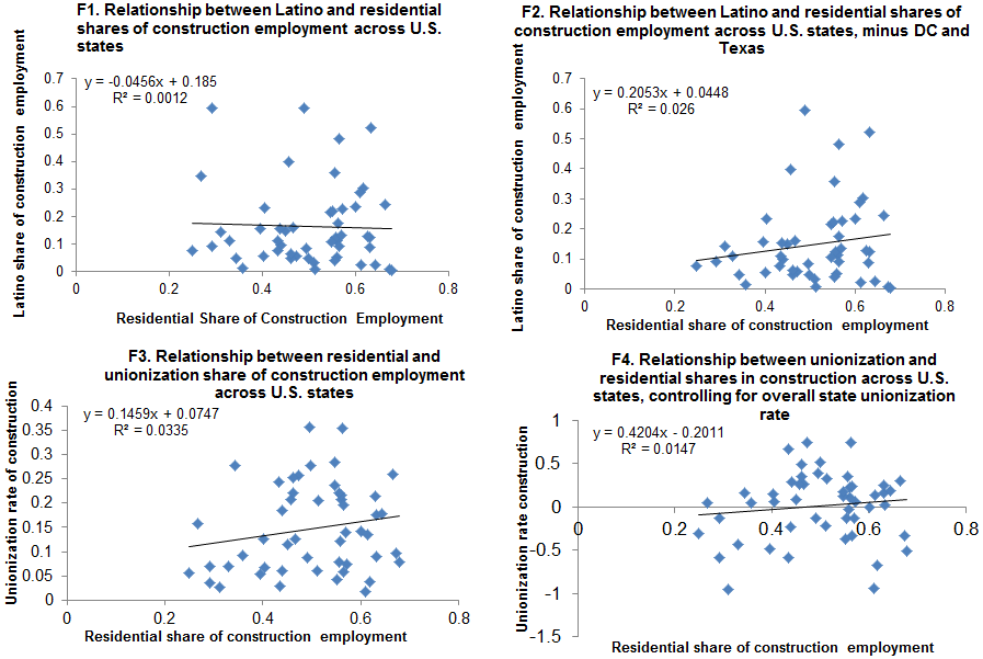
Next, we test to see if the relationships (or lack thereof) in the simple bivariate scatterplots hold up in multivariate regressions. We run regressions that examine the correlation between the Latino share of overall construction employment and the share of the construction workforce that is unionized in a given state and the residential share of construction employment.
Table 11 shows the results from multivariate regression testing the relationships in the scatterplots for robustness. It adds a number of controls to examine whether or not the bivariate relationships examined in Figure F continue to hold.
Testing for bias in demographic outcomes of construction investments
| 1 | 2 | 3 | 4 | 5 | 6 | |
|---|---|---|---|---|---|---|
| Dependent variable | Hispanic share of construction | Hispanic share of construction | Young Hispanic share of construction | Young Hispanic share of construction | Unionization rate of construction | Unionization rate of construction |
| Residential share | 0.69 | 0.084 | 0.72 | 0.19 | -0.84 | -0.73 |
| (3.18)* | (1.28) | (1.58) | (0.28) | (-4.50)* | (-2.84)* | |
| State dummies | yes | yes | yes | yes | yes | yes |
| State-specific time trend | yes | yes | yes | yes | yes | yes |
| National time trend | yes | yes | yes | yes | yes | yes |
| Overall state share (either Hispanic or union) | no | yes | no | yes | no | yes |
| R2 | 0.917 | 0.918 | 0.956 | 0.957 | 0.89 | 0.891 |
| Observations | 588 | 588 | 119 | 119 | 607 | 607 |
| DOF | 484 | 474 | 97 | 87 | 503 | 493 |
* Denotes significance at 5% level.
Source: Author's analysis of data from the Quarterly Census on Employment and Wages (QCEW), as described in text
Results on Latino share of population
Specifically, the regression in column (1) relates the Latino share of construction employment to the residential share of construction employment and includes state unemployment rates, state and year fixed effects, and a state-specific time trend.
The coefficient on the residential share of construction employment is economically significant, but does not pass conventional thresholds of statistical significance (significant only at the 25 percent threshold). Moreover, we should account for the possibility that high shares of residential construction may be associated with overall Latino population in a state, not just construction workers. This check is particularly important if rising Latino population shares actually cause higher rates of residential investment.
Including this state Latino population share reduces the size of the coefficient on the residential share of construction employment, as shown in Column (2).
It is certainly possible, of course, that this examination can miss ways in which a larger residential share in overall construction could have a higher share of Latino employment than the nonresidential sector. We control for a state’s overall population that is Latino in our regressions. But if, for example, Latino workers are disproportionately mobile across state lines and actively seek work in residential employment, then both the Latino share of state population and the Latino share in residential employment would rise as workers moved to find residential construction jobs.
We assessed this by looking at the share of young Latino men in construction as our dependent variable, and use only the overall Latino share in the state’s population in our list of controls. If it is young Latino men searching for residential construction who are more mobile than other Latino groups, then by controlling only for overall Latino population in a state, one can still allow this “job chasing” to boost Latino shares in construction employment when residential shares of construction are larger. However, our results essentially mirrored our earlier regressions (shown in Columns (3) and (4)).
Results on unionization
The results are different, however, for testing whether or not high shares of residential employment in the overall construction sector might bias estimates of unionization rates of nonresidential construction. Column (5) shows the results of a regression that has the state-level unionization rate of the construction sector as the dependent variable. Independent variables include the overall state unionization rate, the state unemployment rate, a state and year fixed effect, and a state-specific time trend. The coefficient on the residential share of construction employment is negative and statistically significant. Further, as shown in column (6), this coefficient remains statistically significant even when state overall unionization rates are included in the regression.
Because the effect of residential shares of construction employment on Latino shares of construction employment did not pass standard statistical thresholds for significance, we do not make any allowance for how the types of jobs created by nonresidential construction (i.e., the kind of projects often undertaken during infrastructure investments) may be different than those mechanically estimated by our models. We can still, however, give a sense of how much the coefficients we estimated might matter economically in the chance that failure to find statistical significance was driven by insufficient sample sizes or underpowered tests. The relative stability of the coefficient on residential construction through various specifications makes us think this is worth doing.
The coefficient estimates from column (2) suggest that each 1 percent increase in the residential share of construction employment leads to roughly a 0.1 percent (.084 in the table) increase in the Latino share of overall construction. Nationally, the residential share of construction employment is almost exactly 50 percent. If one wanted to know what would happen to the Latino share of construction employment in projects that were 100 percent nonresidential, one would simply reduce the Latino share of employment by 10 percent. Given the overall national average Latino share in construction employment of 16.2 percent in 2012, this translates into a 1.6 percentage-point reduction in the share of employment generated through infrastructure projects that is accounted for by Latinos, relative to what is generated by our input-output model in this paper.
More relevantly (because it was statistically significant), the coefficient relating the residential share of construction employment to unionization can also be used to provide an adjustment to the previous estimates in this paper regarding the share of jobs created through infrastructure investments that are unionized. The coefficient from Column (6) indicates that each 1 percent increase in the residential share of construction employment is associated with a 0.73 percent decrease in the unionization rate. Again, taking the fact that today’s residential/nonresidential employment share is 50/50, a series of infrastructure projects that were entirely nonresidential would boost the unionization rate by 73 percent relative to what would be estimated through our input-output model. Given the current unionization rate in construction of 15 percent, this would imply roughly a 10 percentage-point increase in unionization rates relative to our input-output model results. This is clearly an economically significant difference.
Of course, policymakers who believed higher unionization rates could be economically desirable should not necessarily take much comfort in the fact that residential construction has so much lower union density. The degree of unionization—both nationwide and by sector—is strongly influenced by national policy (see Schmitt and Mitukiewicz 2012 on this). But infrastructure investment is not particularly well-suited to affecting the degree of unionization.
Issues regarding the optimal financing of infrastructure investments
As noted previously, if the goal is to increase economic activity and employment in a slack economy, the optimal mode of financing infrastructure investments in the near term clearly is with increased public-sector debt. However, it is generally thought that other forms of government spending that serve as effective economic stimulus when deficit-financed during times of economic slack (transfer payments directed to lower-income households, for example) should be made deficit-neutral if they are to be continued during times of normal economic functioning.
In the United States, the clearest example of this rule regarding “pay-fors” can be seen in the construction of the Affordable Care Act (ACA), often known simply as “health reform.” In this case, even though the ACA was legislated during times of extraordinary economic weakness in 2010, the architects of it ensured that the entire cost of the ACA was more than paid for in the 10-year budget window.
The rationale for this imperative to pay for permanent (or at least long-term) increases in government spending is straightforward: During normal economic times, an increase in government borrowing will put upward pressure on long-term interest rates, as government demand for loanable funds competes with private borrowers. This increase in long-term interest rates can threaten to “crowd out” a range of private investment projects, lowering the potential size of the private capital stock and reducing productivity growth.
However, this logic does not apply so forcefully to permanent (or long-term) increases in public investments (including infrastructure). Even if these are deficit-financed and do indeed lead to some crowding out of private capital investments, as long as the marginal public investments are as productive as the marginal private investments that were crowded out, overall productivity growth is unaffected. Given the falling ratio of public to private capital stocks in recent decades, it seems quite possible that marginal public investments will have rates of return that are competitive with (if not exceeding) marginal private investments. Further, if public capital formation is complementary with private capital formation (as is found in much research), then a boost in the level of infrastructure investments might lead to a “crowding in” of private investments.
Making infrastructure investments “deficit-neutral” also carries economic costs
This recognition of the deep flaws in the conventional wisdom insisting that all increases in public spending be fully paid for in deficit terms informs such actions as past calls for separate capital and current accounts in the U.S. federal budget. Further, it is explicitly acknowledged in the “golden rules of budgeting” released by the Treasury of the United Kingdom in the late 1990s, which stated that government consumption spending should be balanced with revenue over the business cycle, but that borrowing for public investments may be deficit-financed.
The recognition that public investments can raise productivity growth even if deficit-financed becomes even more salient when one considers that the alternative to debt financing often carries economic costs of its own. Taxation is the most commonly considered alternative to debt financing, and taxation is clearly not “free” in terms of economic costs. Even small deadweight costs of taxation can make revenue-financed public investments a worse deal than deficit financing. Of course, taxation of harmful externalities is clearly good policy in and of itself, regardless of what these taxes finance.
While this report has focused on “core” infrastructure investments, it is important to note that often the dividing line between what is a public “investment” versus “consumption” can be blurry, and erring too much on the side of classifying public spending as consumption can lead to suboptimal policy responses. Take the biggest category of public spending: transfers to individuals. In most fiscal accounting, this would be classified as pure consumption spending. As such, if one focused mechanically on boosting the rate of measured productivity growth, it would seem to make theoretical economic sense to finance increases in public investments (infrastructure) with cutbacks to government transfers.
However, a growing body of research has pointed out the substantial economic gains that result from wide swathes of transfer spending (see Bivens 2012b for an extended analysis of the rates of return from “non-core” public investments). Spending on nutrition assistance, for example, can be both economically and fiscally beneficial in the long run because it is an investment in children’s healthy physical and mental development. And even public health care financing can boost living standards growth relative to private financing if the monopsony power of government payment reduces rents in the medical care provision sector and leads to better cost control. So, even besides the normative implications of cutting transfer payments to finance public investment, one should examine very carefully the implicit rate of return even of spending classified as pure transfers before assuming that this method of infrastructure finance is clearly better than either deficit- or revenue-financed spending.
So far, the discussion in this section has involved a number of cautions about financing stepped-up infrastructure investments with instruments (increased revenue or cuts to other government spending, particularly transfers) that may reduce living standards of households. However, it should also be noted that because infrastructure investments have the potential to provide benefits progressively, even investments that are financed directly by user fees may well be a net plus for such households. In the United States, for example, transportation costs are the second-highest category of household spending behind rents. And the share of household budgets accounted for by transportation costs are much higher for the bottom 90 percent of households than for the top 10 percent (see Walsh et al. 2011). Given this, infrastructure investments that can reduce the cost of transportation significantly—say, by providing public transit options or by repairing highways so that automobiles do not require as frequent repairs—will provide benefits that are progressively distributed.
Even from the perspective of aggregate economic efficiency, the optimal mode of financing infrastructure investments is far from clear. Conventional wisdom about government spending (that any long-term increase always needs to be made deficit neutral) is clearly wrong, and even some propositions that are firmly accepted by professional economists (that financing public investments by cutting government transfers will boost prospects for aggregate living standards growth) may well be wrong. But given the extraordinarily large rise in income inequality in recent decades in the United States, we would argue that focusing just on aggregate economic efficiency is far too narrow. The link between aggregate productivity growth and living standards growth for the vast majority has weakened enormously in recent decades. Given the nature of public investments and infrastructure spending, they seem to us a prime opportunity to ensure that some of the benefits of economic growth can be enjoyed by a wider swath of American households than have benefited from trends in market income growth in recent decades. Policymakers should not shy away from analyzing this redistributive effect of infrastructure spending and its optimal financing and making normative judgments about this spending and financing.
Climate economics argues strongly for deficit-financing public investments
There is, moreover, one issue regarding infrastructure investments and redistribution that pure positive economics can prove useful in analyzing: the degree of “sacrifice” required of present generations to begin mitigation of carbon emissions to slow global climate change and bequeath future generations a much-reduced likelihood of climate catastrophes. In much of the economics literature regarding this issue, the degree of current “sacrifice” is assumed to depend upon the discount rate. The larger the discount rate, the less current generations should sacrifice.
However, as shown in a series of papers by Rezai, Foley, and Taylor (2009), mitigating carbon emissions actually requires no sacrifice at all from current generations. Carbon emissions are an unpriced externality, so correcting for this externality only increases the economy’s intertemporal production possibilities frontier (PPF), making any requirement of generational sacrifice unnecessary. Intuitively, what this means is that today’s generation can invest more in carbon mitigation while keeping current consumption unchanged simply by investing less in conventional capital stock.
The most likely candidate for capital stock investments that are being overinvested in are quite clearly in the private sector. Private capital investments are driven strongly by assessments of profitability and hence relative prices. But it is exactly these relative prices that are “wrong” because of the unpriced externality of carbon emissions. On the other hand, public capital investment decisions are much less directly connected to issues of profitability and relative prices, and so are much less likely to have been overinvested in due to the unpriced externality of GHG emissions.
There are many ways theoretically to engineer this expenditure-switching from conventional capital to capital that mitigates carbon emissions, but in practice one way seems obvious: Finance public investments—including infrastructure investments—that mitigate carbon emissions by increasing budget deficits that will crowd out some conventional capital stock investments. It’s important to note that this is not a normative result: The expenditure switch from conventional capital to carbon-mitigating investments is clearly efficient in the positive sense. And, this method of accommodating this expenditure switch is also efficient; by deficit-financing the investments in carbon mitigation and placing upward pressure on interest rates, the conventional capital investments that will be forgone are those with the lowest rates of return.
The impact of infrastructure investments on growth and macroeconomic stabilization
Besides boosting the potential for broad-based living standards growth, an acceleration of productivity carries other potential benefits as well. A number of researchers have identified the acceleration of productivity growth in the late 1990s as a key reason why estimates of the non-accelerating inflation rate of unemployment (NAIRU) fell over this period. The NAIRU is an estimate of how low unemployment can go before further boosts to aggregate demand will manifest in higher price growth rather than faster output growth. In the years leading up to the late-1990s boom, estimates of the NAIRU for the United States had risen to well over 5 percent, and sometimes close to 6 percent, meaning that policymakers (particularly the Federal Reserve) were prepared to slow economic growth through contractionary macroeconomic policies if the unemployment rate threatened to go below this threshold.
Further, this was not an idle threat. Between 1979 and 1995, the actual unemployment rate exceeded the estimated NAIRU by more than 30 percentage points cumulatively—and not just during official recessions.
Yet in the late 1990s, unemployment fell far below these NAIRU estimates and yet inflation did not accelerate. Instead, millions of American workers were employed who would not have been had policymakers put on the brakes when unemployment passed below ex ante estimates of the NAIRU, and American wages saw their first across-the-board period of growth in a generation. This episode highlights two things.
First, the idea that a well-estimated NAIRU can ever be a good guidepost for policymakers should be reexamined and likely abandoned. Besides the U.S. episode between 1979 and 1995, it is quite likely that many large Western European economies also suffered through a decade or more of excess unemployment because the monetary authorities in these countries similarly strove too hard to not allow the overall unemployment rate reach too-conservative NAIRU targets.
Second, however important it is to do away with the concept of a well-estimated NAIRU as a reliable ex ante guide to policy, it remains the case that in the near future official estimates of the NAIRU will likely be vitally important to what policymakers do. If these estimates are too high, then millions of potential work years and hundreds of billions of potential wage earnings for low- and moderate-income workers could be sacrificed.
One must stress that it is the estimated value of the NAIRU that is important, not whether a hard and fast NAIRU actually exists or what its actual (as opposed to estimated) value is. This is because even if there is no firm NAIRU, as long as policymakers think that there is and aim to keep the unemployment rate from breaching it, then great economic gains can be had by lowering the estimated value of the NAIRU. To put it bluntly, as long as the U.S. Federal Reserve thinks it knows the value of the NAIRU, this makes it extraordinarily unlikely that unemployment will be allowed to drift beneath it. Given this, what the U.S. Federal Reserve estimates the NAIRU to be becomes extraordinarily important.
An acceleration of productivity, particularly when preceded by a period of sluggish wage growth, has the potential to significantly reduce the estimated NAIRU. In perfectly flexible labor markets, an acceleration of productivity growth would be accompanied by an equal acceleration of wage demands. However, as a long line of research, summarized by Ball and Mankiw (2002) has pointed out, workers’ wage aspirations are likely inertial. So, when hourly wage growth averaged far less than 1 percent per year for the period between 1979 and 1995, this became the accustomed pace of wage growth for these workers. When productivity began accelerating in 1995, however, this opened up a large and growing wedge between wage aspirations and productivity growth, providing more room for unemployment to fall without sparking wage-push inflation.
It should be noted that the conditions for an acceleration of productivity to push down the estimated NAIRU clearly exist today. Productivity has slowed dramatically in recent years, with average productivity growth between the beginning of the Great Recession through the first half of 2013 essentially matching the 1979 to 1995 pace that has often been dubbed the “Great Productivity Slowdown.” Further, wage aspirations for American workers are clearly at rock-bottom levels. The bottom 80 percent of American workers saw inflation-adjusted declines in wages in each of 2010, 2011, 2012, and the first half of 2013.
Further, the potential for an ambitious investment effort in infrastructure to boost measured productivity levels is real. Bivens (2012a) estimated that an effort that boosted infrastructure investments by $250 billion per year for an extended period would boost measured productivity growth by roughly 0.3 percent per year—more than half the acceleration seen in the late 1990s that was associated with the information and communications technology (ICT) investment boom.
Given the very large downward adjustments to estimates of the NAIRU during the late 1990s ICT boom, as well as the conditions prevailing in the U.S. economy today (specifically, low rates of productivity growth and very low wage aspirations on the part of most American workers), it does not seem unreasonable to think that an ambitious public investment agenda focused on infrastructure spending over the next decade could lower the estimated NAIRU by a percentage point over that decade. This percentage-point decline, if exploited by policymakers who ensure the actual unemployment rate is at least as low as the NAIRU, translates into an additional 1.4 million employed Americans each year and to significantly higher wage growth even for those workers who would have been employed over the decade anyway.
Conclusion
This report has analyzed the potential effectiveness of increasing infrastructure investments as a means to alleviate large economic challenges facing the U.S. economy in the short and long run.
In the short run, this pressing challenge is the failure to make significant progress in spurring a full recovery from the Great Recession. As of the end of 2013, key measures of labor market recovery, such as the employment-to-population ratio of prime-age adults, had recovered just a fifth of the decline experienced during the Great Recession. Further, overwhelming evidence exists that the wedge between actual economic activity and employment levels and levels that would prevail in a healthy economy is nearly entirely a function of deficient aggregate demand.
Infrastructure spending, particularly if deficit-financed, is routinely found by macroeconomic modelers to be among the most effective tools in pushing the economy back toward full employment. Any policy that aims to blunt the impact of infrastructure investment on federal budget deficits will also blunt its impacts in spurring recovery, but infrastructure investments financed by nearly any means besides cuts to transfer spending (i.e., unemployment insurance, safety net programs, and social insurance programs such as Social Security and Medicare) will still provide a substantial boost to economic activity and employment.
In the longer term, some of the U.S. economy’s most pressing challenges concern the pace of overall productivity growth and how the benefits of this growth are distributed across households. After an acceleration of productivity growth beginning in 1995, the years before and since the Great Recession have seen a relatively steady decline in the pace of growth. Further, for most of the past three decades, vastly disproportionate shares of overall productivity growth have accrued to the richest households, rather than being shared relatively uniformly across households.
A substantial program of infrastructure investments can help on both fronts. A long literature (some of it quite recent) has identified strong impacts of infrastructure investments on spurring overall productivity growth. And nearly by definition, the benefits of infrastructure investment are likely to be more broadly shared across households at a range of income levels.
Another (related) long-term challenge the U.S. economy faces is ensuring access to high-quality jobs for traditionally disadvantaged segments of the labor market: women, minorities, workers without a four-year college degree, and young workers. A key question for policymakers is whether or not infrastructure investments could be expected to provide high-quality jobs for such groups without any other policy action to ensure that it does. This report has examined three scenarios of infrastructure investments in the U.S. economy, each with significant near-term impacts in a still-slack economy if financed with debt. The first scenario examines the potential boost to infrastructure spending made possible by cancelling the budget “sequester” that would otherwise automatically reduce spending levels over the next decade. It would generate $30 billion annually in additional infrastructure over the next decade and create 360,000 jobs at the end of the first year. The second scenario examines infrastructure investments that combine substantial upgrades to residential and commercial building efficiency along with an upfront investment in constructing a national smart grid. It would generate $92 billion annually over the next decade, creating 1.1 million jobs. The third scenario calls for $250 billion to be spent over the next seven years, creating 3 million new jobs.
Making these stepped-up infrastructure investments deficit-neutral reduces their boost to near-term activity and employment, though they are still net boosts to activity and employment under any method of financing except for cutting government transfers.
The estimates of near-term impacts are admittedly imprecise. For example, macroeconomic multipliers used by private-sector forecasters and official government agencies are not fine-grained enough to vary significantly across different types of infrastructure spending. This is simply because there is not enough exogenous variation in the data regarding these different types of projects to allow fine-grained differences in economic multipliers to be estimated.
This report noted that the labor intensity of infrastructure projects in the United States tends to be lower than economy-wide averages. This is due mostly (directly or indirectly) to the very low labor intensity of U.S. manufacturing. A key driver of this low labor intensity in U.S. manufacturing, however, is specialization driven by globalization. This specialization, however, will work in reverse for many countries in the global South, so one should be very careful indeed in assuming that what holds in data regarding the labor intensity of U.S. infrastructure spending will also hold for other countries.
While there are not enough data to provide precise estimates, a number of careful researchers have suggested that infrastructure maintenance projects (or, an emphasis on “fix it first”) may well be more labor-intensive than new construction. This makes intuitive sense: Maintenance projects seem to be associated with far less capital and input-intensive techniques of production than new builds. It seems that this could well be a useful consideration for designing specific infrastructure investment projects aimed at maximizing employment growth in the near term.
In the longer term, even if such investments do not lead to net new jobs created because of countervailing macroeconomic influences, they will still significantly change the composition of labor demand in the U.S. economy. Specifically, the jobs generated through such investments are disproportionately male, disproportionately Latino, disproportionately require less than a four-year college degree, disproportionately middle- and high-wage, and skew away from younger workers.
In terms of many employment and social goals that might plausibly be met through infrastructure spending, this is a mixed bag of results. Spurring employment opportunities for non-white workers in the U.S. economy is a laudable goal, and infrastructure projects do indeed skew toward Hispanic, non-white workers. However, employment generated through these projects skews away from black workers, and overall infrastructure investments do not generate employment that skews toward non-white workers generally.
Similarly, infrastructure investments tend to generate employment that skews very heavily male. For those concerned generally about securing equal access to occupations for women, this could seem like a strike against such investments as employment policy.
Finally, on the downside, infrastructure investments generate jobs disproportionately for workers older than 25. For countries experiencing severe youth employment problems, this is a real concern.
However, these genuine concerns could argue more strongly for creating complementary policies to infrastructure investments, rather than arguing simply for not undertaking these investments, the latter of which would, of course, do damage well beyond employment outcomes. For example, regulatory, policy, and legal levers should be used to ensure that jobs in construction and manufacturing are indeed open to workers of all genders, races, and ethnicities. And in the United States, the lack of young workers in construction and manufacturing could well argue that the country’s apprenticeship programs are sorely lacking and need modernization and support.
But some of the news about the employment outcomes that would be expected from infrastructure investments even without complementary policies can be seen as hopeful. For one, the jobs generated would boost demand for workers without a four-year university degree. This is a group that in the United States in recent decades has seen the worst wage outcomes, so anything boosting demand for their labor would be a positive. Importantly, this group remains the large majority of American workers.
Further, the jobs generated by infrastructure investment are predominantly middle-wage jobs—and the share of jobs generated in the bottom quintile is very small. This is most welcome in an economy that has had extraordinary difficulty in generating decent jobs for most of the labor force in the past decade.
Besides their direct impacts on the labor market, an increase in infrastructure investments has been shown by a large and growing research literature to yield large economic returns and carry the potential to boost productivity growth. Given the sharp deceleration in U.S. productivity growth since the beginning of the Great Recession, this effect alone could justify additional infrastructure investments over the next decade.
Even more importantly, if this boost in productivity led (as it did in the late 1990s) to a drifting down of policymakers’ estimate of the NAIRU, and if this lower estimated NAIRU led to more expansionary macroeconomic policy, this would be a huge win for employment generation across the board. Further, because traditionally disadvantaged workers (non-white minorities, workers without a four-year college degree, and young workers particularly) benefit the most from any reduction in overall unemployment, infrastructure investments that boost overall productivity carry the potential to also hit many social and employment goals.
All in all, if policymakers were determined to ensure that any spending flow directly employed as much labor as possible in the U.S. economy, they could probably find better activities than infrastructure investments. But given the large potential benefits of infrastructure investments stemming from its boost to productivity growth, macroeconomic stabilization, and job quality, and given as well that any direct (and supplier) employment generation disadvantage is quite mild, concerns about employment generation should certainly not preclude infrastructure investments in the United States. Further, developing countries assessing the impacts of infrastructure spending should take heart that much of the labor-intensity disadvantage of infrastructure investment may be particular to the United States (and maybe its advanced-country peers).
About the author
Josh Bivens joined the Economic Policy Institute in 2002 and is currently the director of research and policy. His primary areas of research include macroeconomics, social insurance, and globalization. He has authored or co-authored three books (including The State of Working America, 12th Edition) while working at EPI, edited another, and has written numerous research papers, including for academic journals. He appears often in media outlets to offer economic commentary and has testified several times before the U.S. Congress. He earned his Ph.D. from The New School for Social Research.
Acknowledgments
This work was prepared for a project undertaken by the International Labour Organization (ILO) to study the employment impacts of infrastructure spending. Financial support from the ILO is gratefully acknowledged.
Appendix: Macroeconomic multipliers
Since the Great Recession of 2008 and the attendant brief resurgence of fiscal policy as a macroeconomic stabilization tool, there has been an ongoing debate about the size of fiscal multipliers: how much economic activity (GDP) is spurred by an increase in government spending.
The broadest case that public spending can boost economic activity comes directly from the accounting identity for GDP (identified as national output, or Y, in the identity below):
(1) Y = Consumption Spending (or, C) + Investment (I) + Government spending (G) + Net exports (X-M)
Increasing government spending directly increases gross domestic product, per (1). Further, it is theoretically possible that each dollar of increased government spending (or tax cuts) can lead to more than a dollar of increased economic output. The intuition is simply that if, say, $100 is spent by the government to employ new street cleaners, these cleaners will spend this income buying, say, food and clothing. This boosts the income of food and clothing retailers, who can then go out and increase their spending on other items. This iterative process is often referred to in macroeconomics textbooks as the “multiplier effect” of fiscal support, and it is driven simply by the fact that consumption spending is both a component of and is itself a function of overall income.
We can express this by having consumption spending be composed of an autonomous component (C0) and a component that depends on disposable (that is, after-tax) income (c(1-t)Y). This allows us to rewrite our identity for GDP as:
(2) Y = A + MPC*Y, where A is simply C0 + I + G + (X–M), and the MPC (or marginal propensity to consume) is simply c(1-t).
Rearranging terms gives us the following expression for Y:
(3) Y = A/(1-MPC)
From here, changes in autonomous expenditures (including G) will boost GDP by an amount equal to their change multiplied by 1/(1-MPC). The higher is the MPC, the larger is the multiplier. It is largely differences in the MPC that lead to differences in estimated multipliers for different sorts of fiscal support. Support aimed at low-income households and direct government spending for infrastructure projects, for example, are often thought to have higher multipliers, as less money “leaks” out of aggregate demand because savings rates are either zero (infrastructure spending) or quite low (low-income households tend to spend a much larger share of any incremental gain to income than higher-income households).4
Textbook macroeconomics clearly teaches that the most effective way to use discretionary fiscal policy to boost economic activity is to finance this support with increased debt. If increased government spending (which adds to GDP directly through the accounting identity) is instead financed with increased taxes (which subtract from GDP by reducing households’ disposable personal income and hence reduce consumption spending), then it is much less effective. Because of this, the size of the “fiscal impulse” stemming from discretionary fiscal stabilizations is often measured simply as the increase in the federal budget deficit engendered by a fiscal policy intervention.
However, textbook macroeconomics also clearly teaches that even deficit-financed fiscal policy support may not boost overall GDP in many economic circumstances.
Crowding out
The most-cited reason why deficit-financed fiscal support may fail to boost GDP in many circumstances is often referred to in shorthand as “crowding out.” By increasing its borrowing, the federal government is competing with private-sector borrowers for loanable funds. This increased competition may well raise overall interest rates, and some private-sector borrowers may decide at these higher rates to not engage in the investment or consumption project they would have engaged in at lower rates. Hence, the extra activity spurred by fiscal policy crowds out some degree of private-sector activity by pushing up interest rates. In the extreme, this crowding-out can be complete, leading to no increase at all in economic activity stemming from large increases in fiscal support.5
These simple mechanics of crowding out, however, assume that interest rates move sharply enough, and assume as well that economic activity is responsive enough to these interest rate movements to materially negate the impact of increased fiscal support. However, when overall weakness in the demand for loanable funds (say, in the aftermath of the burst housing bubble) has pushed interest rates all the way down to zero lower-bound (or ZLB), it dims the prospects for fiscal support to completely overwhelm this intense downward private pressure on rates and push interest rates up high enough to begin choking off more privately supported activity than the fiscal support is supporting itself. Yet many arguments expressing skepticism about the efficacy of ARRA leaned clearly on the role of crowding out in rendering it ineffective.6
The importance of the ZLB on interest rates in contemporary debates should be stressed. The primary reason why there was much stronger and more widespread support among macroeconomists for discretionary fiscal support for the economy in 2009 than in any other recession in recent memory is entirely explained by the fact that interest rates were at the zero bound. This bound both constrains the ability of the Federal Reserve to fight recessions with its own conventional tools (and hence adds to the desirability of expanding the portfolio of countercyclical policies), and substantially allays the fear that increased fiscal support will lead to crowding out. If fundamental economic forces have pushed interest rates down to zero (or as close to zero as they can effectively go, in the case of longer-term rates), that should allay fears that increased government borrowing will lead to upward pressure on these rates so intense that it leads to great withdrawal of investment spending in the economy.
Ricardian equivalence
Another argument against the efficacy of discretionary fiscal support concerns the notion of Ricardian equivalence: the notion that an increase in deficits will be recognized by households as a future tax increase, and hence will spur them to increase their own savings to build up wealth to pay these higher future taxes. There are a couple of reasons to doubt that the full Ricardian effect of rising private savings sterilizes increased public dissaving. For one, some of the increased future taxes that will pay back today’s deficits will fall on future generations, so the current generation will indeed see a fall in its lifetime tax burden as a result of the public dissaving. Second, many households (particularly in a downturn associated with financial market distress) may be liquidity-constrained, preferring a marginal dollar of consumer spending over a marginal dollar of savings, but currently unable to borrow. To the extent that public dissaving relieves this constraint, it can increase current spending. Lastly, if the fiscal boost from dissaving comes in the form of spending (say, on infrastructure projects), then there is no reason why private saving should rise to pay off this extra public debt one-for-one in the current year. For example, if the federal government borrows and spends $1,000 per person to build highways this year, households will only have to reduce their spending by (the net present value of) $1,000 over the rest of their lives to pay the higher future taxes that result. So, the Ricardian equivalence mechanisms do not mean that it is impossible for any kind of public dissaving to boost overall spending in a given year.
Timing lags
Besides the mechanics of crowding out and Ricardian offsets, however, the case against discretionary fiscal policy stabilizations has also rested on issues of timing. Because fiscal policy support is often associated with lags both in deliberation (the inside lag) as well as implementation (the outside lag), many macroeconomists have argued that fiscal policy support may arrive too late, that is, after an economic recovery had already spontaneously begun. These arguments went so far as to claim that the fiscal support could arrive late enough to push an economy directly into overheating, leading to inflation and interest rate spikes. Because monetary policy tends to operate with a much-shorter inside lag, recent decades have seen a growing (but not universal) agreement among policymakers and macroeconomists that most recession-fighting responsibilities should be borne by central banks, and not by Congress and the president.7
Ironically, the case against discretionary fiscal stabilizations seems to have achieved its greatest foothold among policymakers and economists just as this crucial timing argument was clearly losing much of its force. While recessions between 1947 and 1990 were indeed quite short and recoveries tended to follow rapidly after business cycle troughs, recessions since 1981 have taken progressively longer time before economic resources were again fully utilized. Given this record, it seems very hard to give credence to worries that fiscal support legislated during a recessionary period will come so late that it will push an already-recovered economy directly into overheating.
Automatic stabilizers versus discretionary policy
We will end this discussion by noting a glaring disconnect between the amount of political controversy surrounding the increase in budget deficits associated with automatic stabilizers and those associated with discretionary fiscal support (say, for example, the ARRA passed in the United States in 2009). From an economic point of view, except for the issues raised by timing lags, deficits are deficits, and if they are desirable or undesirable, one’s analysis should not change based on whether they occur mechanically or through policy changes.
Yet ARRA was a much larger political controversy than the much larger increases in deficits associated with the role of automatic stabilizers during the Great Recession. For example, many criticisms of ARRA leveled by economists opposed to it invoked the problem of crowding out as the reason why it would not work to stabilize economic activity.8
But very few economists (none, in fact, that this author could find) argued in 2008 that the rising budget deficits driven mechanically by the slowing of economic growth should be closed rapidly through policy action. If concerns over crowding out were not thought to apply to these large increases in deficits stemming from automatic stabilizers, then it is far from obvious why they would apply to increases stemming from discretionary fiscal measures either. After all, the market for loanable funds does not know which increment of increased federal government demand for borrowing is discretionary (i.e., legislated specifically to fight an ongoing recession) versus which increment is nondiscretionary (i.e., responses in means- and circumstances-tested programs and progressive marginal tax rates) and cannot respond differently to each. Further, the types of public dissaving associated with rising deficits driven by automatic stabilizers (specifically, falling taxes and increased government transfers) are much more likely to engender a full Ricardian offset from rising private savings in theoretical models (tax cuts in particular are fully sterilized in the most rigid Ricardian models).
The U.S. federal budget deficit rose by more than 9 percent of GDP between 2007 and 2009, but ARRA could only account for a bit over 2 percentage points of this increase; the large bulk of the increase between those years was the automatic outcome of tax revenues falling as economic activity collapsed, and needs-based safety-net spending rising.
Given this near-completely sanguine acceptance among policymakers and applied macroeconomists of the large increases in budget deficits stemming from automatic stabilizers, timing lags associated with discretionary fiscal policy interventions are the only source of worry about the potential effectiveness of ARRA that make much analytical sense. Given the track record of long recoveries from recessions in the early 1990s and early 2000s, and given that as of December 2011—four years after the previous business cycle peak and two-and-a-half years after the official end of the recession—employment remained 5.8 million below the prerecession peak, the timing-lags objections to ARRA are not in retrospect particularly compelling.9
Of course, there is a more cynical reason why many policy analysts had no problem at all with the much-larger increases in budget deficits that predated ARRA: they took place under a different presidential administration.
Multiplier estimates
In recent years, the debate about the size of economic multipliers in the U.S. economy centered almost entirely around the impact of ARRA. Contemporaneous estimates of the effect of infrastructure projects undertaken in a slack economy when the monetary authority was highly likely to fully accommodate the increase in federal debt in the United States relied, understandably enough, on models and estimates of prior fiscal policy interventions. So, for example, when the CBO released its quarterly report on the effect of ARRA on economic activity and employment, it relied on multipliers estimated in this previous literature. This led to some misunderstanding; several critics of the ARRA and increased public spending during recessions claimed that estimates of ARRA’s effect simply reflected “assumptions” made about multipliers by the CBO (or other private-sector forecasters who had quite-similar estimates of its impact). This was not the case: Multipliers (upon which the CBO estimates were based) are not simple assumptions, they are the result of estimations, and these “model-based” estimates of ARRA’s impacts were perfectly valid and, as subsequent econometric work has shown (to be taken up later in this section) actually quite good predictors of the effectiveness of ARRA spending in supporting economic activity. Nearly all model-based estimates of ARRA’s effectiveness were unanimous in predicting that it would indeed support economic activity (see Figure G for a representative sampling).
Estimates of ARRA's boost to U.S. GDP in 2010 Q2 by various sources
| Source | Estimate |
|---|---|
| Zandi/Blinder | 2.7 |
| Congressional Budget Office | 3.15 |
| Council of Economic Advisers | 2.95 |
| Goldman Sachs | 2.6 |
| Global Insight | 2.2 |
| JPMorgan | 3.7 |
| MacroAdvisers | 2.1 |
Note: ARRA stands for the American Recovery and Reinvestment Act of 2009.
Source: Council of Economic Advisers (2011)
Prospective estimates of multipliers: “Average” multipliers are not an appropriate guide
However, it is clearly true that a good estimation of macroeconomic multipliers is challenging. By far the most important first step in obtaining estimates of multipliers that are applicable to the effect of ARRA on the U.S. economy in 2009 and 2010 is to restrict one’s estimates of prior episodes of fiscal policy interventions to those undertaken in similar economic contexts. Importantly, this means situations during which unemployment rates were high and capacity utilization rates were low, as well as situations where interest rates were quite unlikely to rise in response to increased fiscal support, either because the central bank had moved to lean against the fiscal impulse or because private-sector demand was so high that the increase in marginal borrowing done by the federal government rapidly pushed up interest rates.
Many studies did not follow this rule of looking only at fiscal support in these specific conditions. Many studies instead looked at fiscal support undertaken over very long stretches, and unsurprisingly found small average multipliers. But these small averages could well be the result of very large multipliers during times of high unemployment and low interest rates, combined with low (or even negative) multipliers during times of increased fiscal support when unemployment was already low and interest rates high (see Romer 2011 for more on this point).
In short, average multipliers are not useful for answering the questions about ARRA’s effectiveness; instead, only studies of the effect of fiscal support on high-unemployment economies near the ZLB on interest rates are useful.
This obviously rules out some of the more prominent claims about the effectiveness of fiscal policy, such as those of Barro and Redlick (2011). This study looked at increases in deficit-financed government spending undertaken since World War II to obtain an estimate of multipliers. They use military spending as the measure of government spending. Their empirical results are dominated by World War II and Korean War periods, when very large increases in military spending were not accompanied by large increases in economic activity. However, by the onset of World War II the economy enjoyed more-than-full employment; the unemployment rate by 1941 was 4.7 percent, and between 1942 and 1945 unemployment averaged less than 1.5 percent. Further, wage and price controls were passed (in part) to contain inflation that would have resulted from excess aggregate demand.10 Similarly, during the Korean War (1950–1953), the unemployment rate averaged just 3.3 percent.
The simple prescription that multipliers cannot be reliably estimated during times when the economy was close to full employment and when interest rates would rise sharply in response to increased fiscal support is violated in a surprising number of studies invoked in the debate over ARRA’s effectiveness in its first two years. Some notable studies that did not suffer from this problem, however, were Eggertsson (2009); Hall (2009); Ilzetzki, Mendoza, and Vegh (2010); and Woodford (2011). Unsurprisingly, given that they are actually all estimating the central parameter of interest—the effect of fiscal support in depressed economies near the ZLB on interest rates—all these studies find that the multiplier on particular forms of fiscal support (direct government spending, in particular) is well over 1 and often close to 2.
It is also worth noting that the Council of Economic Advisers (CEA) did not just use previously estimated values of economic multipliers to predict the effect of ARRA. They also estimated a vector autoregression (VAR) model to predict what GDP would have been with no fiscal support based on its pre-ARRA trajectory (and historical relationships between key variables) and then compared that prediction with its actual (post-ARRA) performance. This VAR approach predicted effects of ARRA that were in line with those predicted by economic multipliers.
The estimates in this report on the impact of infrastructure investment rely heavily on the CBO and CEA multiplier estimates. As the next section will note, however, these prospective estimates have been largely vindicated by retrospective, more direct empirical estimates of the effect of the components of ARRA.
Retrospective estimates of economic multipliers of the components of ARRA
Now that ARRA has largely run its course, there is now actual data to try to test to see if one can directly estimate its impact on economic activity. Again, however, this is much harder to do than is often recognized. The problem, in the jargon of econometrics, is how to gain “clean identification” of ARRA’s impact. Take, for example, one obvious (but naïve) way to glean its effects: Compare states that have gained more ARRA funding than others to see if economic conditions improved more significantly in those high-ARRA-aid states. The problem with this approach is that much ARRA funding (expanded unemployment insurance and food stamps, for example) was contingent on economic circumstances, with more money mechanically going to states that have a bigger contraction of economic activity. Simply examining correlations between state-level spending and economic activity could well find a negative correlation, but one that is driven by a chain of causality that runs from depressed economic activity to more ARRA funds.
The chief challenge in many attempts to estimate the impact of ARRA is to precisely find ways around this problem of reverse causality, and this is the problem of “clean identification.”
A series of attempts to do this came from John B. Taylor (2011), who used aggregate time series evidence on personal income and consumption to estimate the impact of the tax rebates and some social transfers (particularly the increase in unemployment benefits) contained in ARRA, along with tax rebates that were passed in 2001 and 2008 in the name of providing fiscal support to the economy. Taylor used these results to argue that one could not reject the hypothesis that the tax rebates and transfers had no impact on personal consumption spending.
Taylor (2011) runs a time-series regression of personal consumption expenditures (PCE) as the dependent variable. As explanatory variables he includes “stimulus payments” and disposable personal income minus stimulus payments, with controls for oil prices and net worth lagged two quarters. His sample period runs from the first quarter of 2001 to the first quarter of 2011. As the coefficient on stimulus payments does not register as statistically significant at the 95 percent confidence level, Taylor takes this as evidence stimulus payments did not work, i.e., that they did not boost consumption spending and hence failed to provide support to overall economic activity.11
However, Baker and Rosnick (2012) show that Taylor’s results are largely driven by the period after the fourth quarter of 2008. More specifically, the ARRA tax rebates and transfers took place in the midst of a collapse in overall spending and against the backdrop of a financial crisis. When they add a dummy variable for the post-2007 period to the same time-series regression run by Taylor (2011), they find that stimulus payments are both statistically and economically significant determinants of consumption spending.
A number of papers try to exploit the state-level variation in ARRA payments to assess ARRA’s economic impact. Again, the key challenge in doing this is to avoid the problem of endogeneity of state receipts—that is, the problem of states with the most depressed economic activity receiving more ARRA funds by design. What is good stabilization policy (focusing more money on more depressed areas) makes for quite difficult evaluation.
Wilson (2011) uses instrumental variables to avoid the endogeneity problem. All of them seek to isolate the purely exogenous portion of ARRA fiscal relief allocated to state governments. For example, the increased aid ARRA provided states for Medicaid payments during the recession was allocated based on a formula that made this aid a function of the prerecession Medicaid share paid by a state, a “hold harmless” component of funding that is based on the three prior years of state per capita income growth, and the change in the state unemployment rate. Through controls in his regression (say, by including the change in state unemployment), Wilson is able to isolate that component of increased state aid that is orthogonal to its economic performance. Beside the Medicaid formula, Wilson also isolates the exogenous components of Departments of Transportation and Education aid to states associated with ARRA. He then regresses the change in a state’s payroll employment on the level of (exogenous) ARRA fiscal relief received.
Wilson (2011) finds that the ARRA fiscal relief is positively correlated to state employment growth, and the result is both economically and statistically significantly (as well as robust to different specifications). He finds that ARRA’s peak impact on employment (he does not use state-level measures of GDP) occurred in the first quarter of 2010, when it was associated with employment levels in that quarter that were roughly 2 to 2.9 million jobs higher than would have been the case absent ARRA’s support. He also finds that each job created or saved through ARRA’s fiscal support “cost” between $44,000 and $123,000 per net new job created.
Feyrer and Sacerdote (2011) also use state-level variation in ARRA spending flows to estimate its impact. They, like Wilson (2011), also utilize instrumental variables to control for endogeneity of ARRA state spending. The instruments Feyrer and Sacerdote (2011) utilize are mean seniority of the state’s delegation in the U.S. House of Representatives and the size of the state’s population. The first instrument, the mean seniority of the state’s House delegation, is assumed to be positively correlated with state-level ARRA spending because a more senior delegation is thought to be able to steer more resources toward its state. The second instrument, state population, is assumed to be negatively correlated with ARRA spending flows. One rationale for this is that the structure of the Senate (with each state, regardless of size, having the same representation) tends to favor small states. Another rationale put forward by Feyrer and Sacerdote (2011) is that smaller states have more miles of roads and highways per capita; because much of ARRA’s direct spending was directed toward highway funds, this results in more funds being directed toward the smaller states. Whatever the precise mechanism of the inverse relationship between state population and per capita ARRA spending, it holds in the data. Further, because both instruments—mean seniority of the House delegation and state population—are clearly driven by historical trends that predate the Great Recession, they are unlikely to be systematically correlated with macroeconomic performance in the state during 2009 and 2010.
The Feyrer and Sacerdote (2011) results are not precisely estimated (the overall multiplier for the stimulus package in various specifications runs from 0.5 to 2), but across a wide range of specifications the results are positive and statistically significantly different from zero.
Chodorow-Reich et al. (2012) also use state-level variation in ARRA spending to test ARRA’s impact. They also surmount the endogeneity of state ARRA spending by utilizing instrumental variables. The instrument they choose is the component of increased federal Medicaid spending directed toward states that is unrelated to changes in economic circumstances. The formula that determines the amount of federal aid directed toward states for Medicaid is driven by a number of factors that are related to the state of the economy (for example, the change in beneficiaries over the previous period, the change in the unemployment rate in the previous period, and the change in average spending per beneficiary). But the formula is also influenced by the amount of Medicaid spending in the state in the period before the recession began, and this is not plausibly related to subsequent developments in state economies.
The Chodorow-Reich et al. (2012) findings provide the largest positive effects of ARRA on employment outcomes. They find that each $100,000 in Medicaid aid provided through ARRA to the states leads to 3.5 job years created or saved. Given that the Medicaid aid alone in ARRA was nearly $90 billion, this means that this portion of ARRA alone (less than one-eighth the total) could have created more than 3 million job years by itself.
Conley and Dupor (2011) is the last study to use state-level variation in ARRA spending to assess its impacts. Like the others, Conley and Dupor (2011) utilize instrumental variables to assess ARRA’s impact. The instruments they choose are the highway funding components in ARRA, the prerecession ratio of a state’s federal taxes and federal receipts, and the political affiliation of the state’s governor.
Conley and Dupor (2011) find no statistical evidence that ARRA created (or destroyed) private-sector jobs in the aggregate. They instead parse private-sector jobs into three rather unconventional categories: goods-producing; a bundle of service-sector industries that includes health, education, leisure, hospitality, business, and professional services (a bundle they call HELP); and all other non-HELP service industries. Not enough justification is given for this unique parsing of service-sector industries. In their benchmark finding, no industry groupings—none of the private industry groups nor the public sector—show any statistically significant relationship to ARRA spending. In a second specification, which they label “fungibility imposed,” two of the three private-sector groupings (goods-producing industries and HELP services) and the public sector show no statistically significant relationship to ARRA spending, while employment in HELP services is shown to be negatively correlated with ARRA spending flows.
Further, the specific regression estimated by Conley and Dupor (2011) makes their results not directly comparable to the other state-based econometric estimates of the specific impact of ARRA. Instead, their preferred econometric specification uses the difference between state aid received by ARRA and negative state revenue shocks as the key independent variable. This specification seems more appropriate for answering a general question as to how state employment is affected by (net) negative revenue shocks, but, given the state-specific shock, it does not then tell us how ARRA aid specifically impacted employment growth. The simplest way to state the inability to directly compare the Conley and Dupor (2011) studies and those of others in this vein is that the estimated multipliers cannot be compared because the multiplicands are different.
This issue of the size of the multiplicand is also the key issue in regards to Cogan and Taylor (2012). This study does not exploit cross-state variation in ARRA spending to assess its impacts, but instead tries to account for the drag imposed by state and local government spending cutbacks in blunting the overall support to the economy provided by the government sector as a whole. Cogan and Taylor (2012) find that states cut back their own purchases by more than the ARRA provided to them in aid. Noting that state and local spending is fungible with respect to the ARRA flows transferred to state and local governments, Cogan and Taylor (2012) interpret this finding as demonstrating that ARRA did not boost government purchases materially and hence could not have had an effect on economic activity. But again, their paper is about the size of the multiplicand, not the multiplier, of ARRA spending.
Given the failure to find statistically significant results from their measures of ARRA spending net of state and local contraction, neither Cogan and Taylor (2012) nor Conley and Dupor (2011) can actually reject the argument that the simple size of ARRA was insufficient to measurably impact state-level trends in economic activity and employment, and not that the marginal effectiveness of a dollar spent by ARRA was low. This is an important point. Cogan and Taylor (2012) and Conley and Dupor (2011) are essentially assuming that states would not have cut back their own spending as much had ARRA funds not been allocated to them; this is the heart of their argument about fungibility. But, as shown by McNichol (2012), even with the ARRA state aid, state and local governments had very large budget shortfalls in 2009 and 2010 (and indeed are expected to see shortfalls for years to come). Given that most states have balanced budget requirements, this means that one cannot plausibly say that state spending would have been higher in the absence of the ARRA funds. In fact, relative to any plausible counterfactual, state spending must have been higher following the receipt of Recovery Act funds.
To argue that the Cogan and Taylor (2012) and Conley and Dupor (2011) papers are not estimating comparable multipliers to other state-based studies is not to say that their findings are of no note to applied macroeconomists and policymakers. The CBO (2012), for example, has actually reduced its estimate of the likely impact of infrastructure spending increases that are managed through grants to state and local governments precisely because of the worry that these governments will reduce their own spending in response to the grants. However, this does not mean that assessments of the all-else-equal impact of infrastructure spending have been reduced because of economic evidence. Rather, it means that policymakers should strive to ensure (perhaps through maintenance of effort requirements for the receipt of federal grants-in-aid) that state and local governments do not sterilize any of the stimulative effect of grants by reducing their own spending.
The studies of ARRA’s impacts that exploit state-level variation to estimate employment multipliers of ARRA spending all come to the conclusion that the effects are statistically and economically significant. The range of estimated multipliers is fully in line with model-based estimates of ARRA’s impact that are based on past estimation of the effect of fiscal policy, and in fact contain many estimates that are above the high range of these model-based estimates. It is worth noting that this state-based evidence is extraordinarily strong evidence of ARRA’s effectiveness, given the many limitations to measuring ARRA’s impact in this way.
For one, the state-level regression may miss some of ARRA’s impact because while money may have been directed to a specific state and created economic activity, some of the employees hired may well live in other states. If, for example, ARRA funds road improvements in Manhattan, many of the employees working on that project will surely come from New Jersey and Connecticut.
Second, much of the economic activity spurred by the direct spending components of ARRA (infrastructure investments in particular) is quite input-intensive; bulldozers and concrete for building roads, for example. Given this, money spent paving roads in Florida may well have spurred economic activity in bulldozer factories in Ohio and concrete plants in Alabama.
Lastly, much of the re-spending effects of the Recovery Act are also likely to leak across state borders. If highway projects in Arizona provide the purchasing power to construction workers to buy new cars, this second-round spending effect will be felt in automobile-producing states like Michigan, not directly in the receiving state of Arizona.
Summing up: Can we still rely on prospective multipliers included in ARRA?
In the end, what is striking about the actual econometric estimates of the specific effect of the Recovery Act and its components—including infrastructure investments—is how cautious model-based estimates like those of the CBO, CEA, and private-sector forecasters were relative to what was actually estimated. This actually should not be a huge surprise. Economic theory teaches clearly that fiscal support has much larger multiplier effects when economies are deeply depressed, when interest rates are pinned at the ZLB, and when central banks are committed to forestalling any countervailing monetary contraction in the face of the fiscal expansion. For the first time since the Great Depression, all of these conditions held in the U.S. economy of 2009 and 2010.
Given this track record, we remain firmly confident that the multipliers used to estimate near-term impact of infrastructure spending on economic activity and employment are solid.
Endnotes
1. These cuts include not only the well-known budget “sequestration” but also include the discretionary spending caps imposed by the Budget Control Act (BCA) of 2011.
2. The “stabilization wedge” concept was first introduced by Pacala and Socolow and is described in S. Pacala and R. Socolow, “Stabilization Wedges: Solving the Climate Problem for the Next 50 Years with Current Technologies,” Science, August 2004, http://www.sciencemag.org/content/305/5686/968.abstract#aff-1.
3. For our measure of potential GDP, we use the series estimated by the Congressional Budget Office. It is an estimate of what GDP would be if the economy were at the Non-Accelerating Inflation Rate of Unemployment (NAIRU) as estimated by the CBO.
4. For the United States, the simple value of the multiplier is also limited in practice by the fact that a significant portion of marginal expenditures is actually satisfied by imports, which do not add to GDP.
5. This presentation is the closed-economy version of crowding out. It should also be noted that in models with a fixed global interest rate, fiscal support can be crowded out by a one-for-one decrease in net exports stemming from a strengthening of the national currency’s value that follows the increased fiscal support.
6. Cogan et al. (2010), for example, find small multipliers in part because they assume a countervailing response from the central bank, which is an endogenous form of crowding out.
7. Blinder (2006) outlines the timing arguments in some detail. Probably the most famous statement of how countercyclical interventions have the potential to increase economic instability comes from Friedman (1953).
8. For example, in the run-up to ARRA’s passage, John Cochrane (2009) wrote, “If the government borrows a dollar from you, that is a dollar that you do not spend, or that you do not lend to a company to spend on new investment. Every dollar of increased government spending must correspond to one less dollar of private spending. Jobs created by stimulus spending are offset by jobs lost from the decline in private spending.”
9. The experience of Japan—which has seen output gaps nearly continuously for nearly 15 years—is another reason to think that the timing argument against discretionary fiscal stabilizations is much less compelling in the context of severely depressed economies facing the aftermath of burst asset market bubbles.
10. Wage and price controls were also put into place to make sure that key wartime industries had the resources they needed.
11. In a related article, Lewis and Seidman (2012) note that an earlier paper by Taylor (2009) used the same methodology and came to the same conclusion regarding the 2008 tax rebates. Yet Lewis and Seidman (2012) make a good point about the limits of arbitrary thresholds of statistical significance: The Taylor (2009) results on the 2008 stimulus payments are indeed statistically insignificant measured at the 95 percent confidence threshold, but are statistically significant measured at the 94 percent confidence threshold.
References
American Society of Civil Engineers (ASCE). 2013. 2013 Report Card for America’s Infrastructure. http://www.infrastructurereportcard.org/
Baker, Dean, and David Rosnick. 2012. Do Tax Cuts Boost the Economy? Center for Economic Policy and Research working paper.
Ball, Lawrence, and N. Gregory Mankiw. 2002. “The NAIRU in Theory and Practice.” Journal of Economic Perspectives, vol. 16, no. 4, 115–136.
Barro, Robert J., and Charles J. Redlick. 2011. “Macroeconomic Effects from Government Purchases and Taxes.” Quarterly Journal of Economics, vol. 126, no. 1, 51–102.
Bivens, Josh. 2003. Updated Employment Multipliers for the U.S. Economy. Economic Policy Institute, Working Paper #268.
Bivens, Josh. 2011. Method Memo on Estimating the Jobs Impact of Various Policy Changes. Economic Policy Institute. http://www.epi.org/publication/methodology-estimating-jobs-impact/
Bivens, Josh. 2012a. Public Investment: The Next “New Thing” for Powering Economic Growth. Economic Policy Institute, Briefing Paper No. 338. http://www.epi.org/files/2012/bp338-public-investments.pdf
Bivens, Josh. 2012b. More Extraordinary Returns: Public Investment Outside of ‘Core’ Infrastructure. Economic Policy Institute, Briefing Paper No. 348. http://www.epi.org/publication/bp348-public-investments-outside-core-infrastructure/
Bivens, Josh. 2012c. Macroeconomic Effects of Regulatory Changes in Economies with Large Output Gaps: The “Toxics Rule” as an Example. Economic Policy Institute, Working Paper #292. http://www.epi.org/publication/wp292-regulation-output-gaps/
Bivens, Josh. 2013. Why the Bipartisan Commitment to Public Investment Should Go Beyond Mere Rhetoric. Economic Policy Institute, Issue Brief #262. http://www.epi.org/publication/ib362-bipartisan-commitment-to-public-investment/
Blinder, Alan. 2006. “The Case Against the Case Against Discretionary Fiscal Policy.” In R. Kopcke, G. Tootell and R. Triest (eds.), The Macroeconomics of Fiscal Policy, pp. 26–61. Cambridge, Mass.: MIT Press.
Bureau of Economic Analysis (U.S. Department of Commerce) National Income and Product Accounts. Various years. National Income and Product Accounts Tables [data tables]. http://bea.gov/iTable/iTable.cfm?ReqID=9&step=1
Chodorow-Reich, Gabriel, Laura Feiveson, Zachary Liscow, and William Gui Woolston. 2012. “Does State Fiscal Relief During Recessions Increase Employment? Evidence from the American Recovery and Reinvestment Act.” American Economic Journal: Economic Policy, vol. 4, no. 3, 118–145.
Cochrane, John. 2009. Fiscal Stimulus, Fiscal Inflation or Fiscal Fallacies? Version 2.5. University of Chicago, Booth School of Business. http://faculty.chicagobooth.edu/john.cochrane/research/papers/fiscal2.htm
Cogan, John F., Tobias Cwik, John B. Taylor, and Volker Wieland. 2010. “New Keynesian Versus Old Keynesian Government Spending Multipliers.” Journal of Economic Dynamics and Control, vol. 34, 281–295.
Cogan, John F., and John B. Taylor. 2012. “What the Government Purchases Multiplier Actually Multiplied in the 2009 Stimulus Package.” In Government Policies and the Delayed Economic Recovery, Lee Ohanian, John B. Taylor, and Ian J. Wright (eds.). Stanford University: Hoover Press.
Congressional Budget Office. 2012. Estimated Impact of the American Recovery and Reinvestment Act on Employment and Economic Output from October 2011 through December 2011. http://www.cbo.gov/publication/43013
Congressional Progressive Caucus (CPC). 2013. The Back to Work Budget. http://cpc.grijalva.house.gov/back-to-work-budget/
Conley, Timothy, and Bill Dupor. 2011. The American Recovery and Reinvestment Act: Public Sector Jobs Saved, Private Sector Jobs Forestalled. University of Western Ontario and Ohio State University. http://web.econ.ohio-state.edu/dupor/arra10_may11.pdf
Council of Economic Advisers. 2010. The Economic Impact of the American Recovery and Reinvestment Act of 2009: Fourth Quarterly Report. Executive Office of the President. http://www.whitehouse.gov/files/documents/cea_4th_arra_report.pdf
Council of Economic Advisers. 2011. The Economic Impact of the American Recovery and Reinvestment Act of 2009 Seventh Quarterly Report. Executive Office of the President. http://www.whitehouse.gov/sites/default/files/cea_7th_arra_report.pdf
Current Population Survey Outgoing Rotation Group microdata. Various years. Survey conducted by the Bureau of the Census for the Bureau of Labor Statistics [machine-readable microdata file]. Washington D.C.: U.S. Census Bureau.
Current Population Survey public data series. Various years. Aggregate data from basic monthly CPS microdata are available from the Bureau of Labor Statistics through three primary channels: as Historical ‘A’ Tables released with the BLS Employment Situation Summary (http://www.bls.gov/data/#historical-tables), through the Labor Force Statistics Including the National Unemployment Rate database (http://www.bls.gov/cps/#data), and through series reports (http://data.bls.gov/cgi-bin/srgate).
Eggertsson, Gauti. 2009. What Fiscal Policy is Effective at Zero Interest Rates? Federal Reserve Bank of New York Staff Report, No. 402.
Eggertsson, Gauti, and Paul Krugman. 2012. “Debt-Deleveraging and the Liquality Trap: A Fisher-Minsky-Koo Approach.” Quarterly Journal of Economics, vol. 127, no. 3, 1469–1513.
Electric Power Research Institute (EPRI). 2011. Estimating the Costs and Benefits of the Smart Grid: A Preliminary Estimate of the Investment Requirements and Resultant Benefits of a Fully Functioning Smart Grid. Technical Report. http://my.epri.com/portal/server.pt?space=CommunityPage&cached=true&parentname=ObjMgr&parentid=2&control=SetCommunity&CommunityID=405
Feyrer, James, and Bruce Sacerdote. 2011. Did the Stimulus Stimulate? Real Time Estimates of the Effects of the American Recovery and Reinvestment Act. National Bureau of Economic Research Working Paper 16759.
Friedman, Milton. 1953. “The Effects of Full Employment Policy on Economic Stability: A Formal Analysis,” in Essays in Positive Economics. Chicago: University of Chicago Press, 117–132.
Hall, Robert. 2009. By How Much Does GDP Rise If the Government Buys More Output? Brookings Papers on Economic Activity, vol. 40, no. 2.
Ilzetzki, Ethan, Enrique G. Mendoza, and Carlos A. Vegh. 2010. How Big (Small) are Fiscal Multipliers? National Bureau of Economic Research Working Paper #16479. http://papers.nber.org/tmp/591-w16479.pdf
Krugman, Paul. 2013. “Secular Stagnation, Coalmines, Bubbles, and Larry Summers.” The Conscience of a Liberal (New York Times blog), November 16. http://krugman.blogs.nytimes.com/2013/11/16/secular-stagnation-coalmines-bubbles-and-larry-summers/?_php=true&_type=blogs&_r=0
Lewis, Kennth, and Laurence Seidman. 2012. “Did the 2008 Rebate Fail? A Response to Taylor and Feldstein.” Journal of Post-Keynesian Economics, vol. 34, no. 2, 183–204.
McKinsey and Company. 2009. Unlocking Energy Efficiency in the U.S. Economy. http://www.mckinsey.com/client_service/electric_power_and_natural_gas/latest_thinking/unlocking_energy_efficiency_in_the_us_economy
McNichol, Elizabeth. 2012. Out of Balance: Cuts in Services have been States’ Primary Response to Budget Gaps, Harming the Nation’s Economy. Center on Budget and Policy Priorities. http://www.cbpp.org/files/4-18-12sfp.pdf
Murray, Patty. 2013. The Senate Budget. http://www.budget.senate.gov/democratic/index.cfm/senatebudget
Office of Management and Budget (OMB). 2012. “Federal Spending, 2010–2012.” Unpublished data provided by program staff at EPI’s request.
Office of Management and Budget (OMB). 2013. The President’s Budget of the U.S. Government, Fiscal Year 2014. http://www.whitehouse.gov/omb/budget/Overview
Office of Management and Budget (OMB). n.d. Unpublished data provided to EPI in 2012.
Pacala, Stephen, and Robert Socolow. 2004. “Stabilization Wedges: Solving the Climate Problem for the Next 50 Years with Current Technologies.” Science, vol. 305, no. 5484, 968–972. http://www.sciencemag.org/content/305/5686/968.abstract#aff-1
Pollin, Robert, and Heidi Garrett-Peltier. 2011. The U.S. Employment Effects of Military and Domestic Spending Priorities: 2011 Update. Political Economy Research Institute, University of Massachusetts, Amherst. http://www.peri.umass.edu/fileadmin/pdf/published_study/PERI_military_spending_2011.pdf
Pollin, Robert, James Heintz, and Heidi Garrett-Peltier. 2009. The Economic Benefits of Investing in Clean Energy: How the Economic Stimulus Program and New Legislation Can Boost U.S. Economic Growth and Employment. Working paper from the Political Economy Research Institute, University of Massachusetts, Amherst.
Rezai, Armon, Duncan K. Foley, and Lance Taylor. 2009. Global Warming and Economic Externalities. The Schwartz Center for Economic Policy Analysis at The New School, Working Paper 2009-3. http://are.berkeley.edu/courses/envres_seminar/Armon_Rezai.OptimalGrowthwithCC.F09.pdf
Rogers, Joel. 2007. Seizing the Opportunity (for Climate, Jobs and Equity) in Building Energy Efficiency. University of Wisconsin, Madison. http://www.ecy.wa.gov/climatechange/2008CATdocs/IWG/bee/Joel%20Rogers%20-%20Seizing%20the%20Opportunity%20in%20Energy%20Efficiency.pdf
Romer, David. 2011. “What Have We Learned about Fiscal Policy from the Crisis?” Presentation for the Conference on Macro and Growth Policies in the Wake of the Crisis. International Monetary Fund headquarters, March 7, Washington, D.C. http://www.imf.org/external/np/seminars/eng/2011/res/pdf/DR3presentation.pdf
Ryan, Paul. 2013. The Path to Prosperity: The GOP Plan to Balance the Budget by 2023. http://budget.house.gov/fy2014/
Schmitt, John, and Alexandra Mitukiewicz. 2012. Politics Matter: Changes in Unionization Rates in Rich Countries, 1960-2010. Center for Economic Policy Research Report. http://www.cepr.net/documents/publications/unions-oecd-2011-11.pdf
Stern, Nicholas. Stern Review on the Economics of Climate Change. Office of Climate Change, Department of Energy and Climate Change. http://webarchive.nationalarchives.gov.uk/+/http:/www.hm-treasury.gov.uk/sternreview_index.htm
Summers, Lawrence. 2013. “On Secular Stagnation.” Reuters Opinion (blog), December 16. http://blogs.reuters.com/lawrencesummers/2013/12/16/on-secular-stagnation/
Taylor, John B. 2009. The Lack of an Empirical Rationale for a Revival of Discretionary Fiscal Policy. Working Paper, Stanford University.
Taylor, John B. 2011. “An Empirical Analysis of the Revival of Fiscal Activism in the 2000s.” Journal of Economic Literature, vol. 49, no. 3, 686–702. http://www.stanford.edu/~johntayl/JEL_Taylor_Final%20Pages.pdf
Van Hollen, Chris. 2013. House Democratic Budget Alternative. http://democrats.budget.house.gov/issue/fy2014-democratic-budget
Walsh, Jason, Josh Bivens, and Ethan Pollack. 2011. Recovery Act’s Green Investments Create or Save Nearly One Million Jobs. BlueGreen Alliance and Economic Policy Institute. http://www.epi.org/publication/recovery_acts_green_investments_create_or_save_nearly_one_million_jobs/
Wilson, Daniel J. 2011. “Fiscal Spending Jobs Multipliers: Evidence from the 2009 American Recovery and Reinvestment Act.” American Economic Journal: Economic Policy, vol. 4, no. 3, 251–282.
Woodford, Michael. 2011. “Simple Analytics of the Government Expenditure Multiplier.” American Economic Journal: Macroeconomics. vol. 3, 1–35.
Zandi, Mark. 2011. “U.S. Macro Outlook: Compromise Boosts Stimulus.” Moody’s Analytics Economy.com. http://www.economy.com/dismal/article_free.asp?cid=195470
