June 2000 Briefing Paper

THE IMPACT OF THE MINIMUM WAGE

Policy lifts wages, maintains floor for low-wage labor market

by Jared Bernstein and John Schmitt

Welfare reform has focused a great deal of attention on the issue of low-wage work. Even with the low unemployment rates that have prevailed since the late 1990s, the U.S. economy continues to create many low-wage jobs, and even some families that work a substantial number of hours each year are still having difficulty making ends meet.

Increasing the federal minimum wage is one potential policy option for addressing the difficulties these families face. Currently set at $5.15 per hour, the minimum wage covers the vast majority of the low-wage workforce, and sets a wage floor below which no covered worker can be paid.[1] Congress increased the minimum twice in the 1990s and, as of this writing, is considering another increase of $1.00 an hour. Supporters of the minimum wage argue that it does what it is supposed to-lift the wages of those workers with the least bargaining power. Opponents, however, make two basic arguments. First, they claim that the minimum wage costs jobs by pricing low-wage workers out of the labor market. Second, opponents argue that the minimum wage is poorly targeted, since most low-wage workers live in families with relatively high levels of income. An examination of the empirical evidence on low-wage workers and the effects of minimum wage increases reveals that: • No evidence exists that teenagers or less-than-high-school-educated adults lost work as a result of the 1996-97 minimum wage increases. • Historically, analyses of the minimum wage’s impact on young workers have never shown the predicted large job-loss effects. • The small negative employment effects found in past analyses diminish over time and are no longer statistically significant. • Minimum wage increases are well targeted in the sense that 63% of the gains from a dollar increase in the minimum wage would be expected to accrue to working households in the bottom 40% of the income distribution. • Of the 8.4 million workers (age 18 to 64) whose wages and incomes would increase with a one-dollar raise in the minimum wage, 2.7 million (32%) are the parents of 4.7 million children. Of the 2.7 million parents who earned at or near the current minimum wage in 1999, 63% had family incomes below $25,000. • Most minimum wage workers are adults (71%), age 20 and up.[2] Women and minority workers are over-represented among the minimum wage workforce. Slightly less than half (48%) of the minimum wage workforce are full-time workers. We begin by examining the history of the minimum wage over time, relative to both inflation and other wage series. We then turn to an examination of the characteristics of minimum wage workers and compare these to the characteristics of other worker with higher earnings. We then address the question of targeting: to what extent do low-wage workers (the beneficiaries of minimum wage increases) reside in low-income families? Following that, we turn to an investigation of the employment effects of increases, addressing the important question of disemployment. The first set of tests examines the most recent increase by looking at state variation. The second set of tests is based on the variation of the minimum wage over time. We conclude with some policy thoughts based on these findings. The minimum wage over time and characteristics of today’s minimum wage workers

The history of the minimum wage in real terms and relative to other values: Figure 1 shows the inflation-adjusted minimum wage from 1955 to 1999, in 1999 dollars. Since the minimum wage is not indexed (e.g., to inflation or to some measure of wage growth), when Congress fails to increase its value, it declines in real terms. Thus, each uptick in the figure’s graph represents a mandated increase, while the downward trends represent periods when the real value was eroded by inflation. The minimum wage peaked in 1968, when it stood at $7.07 in 1999 dollars.[3] The figure also shows the 30% decline in the minimum wage over the 1980s, when Congress failed to adjust the wage floor for nine years. Even with the recent increases in the 1990s, the inflation-adjusted minimum was 21% lower in 1999 than in 1979. Figure 2 tracks the minimum wage relative to other wage series in order to examine how the trend in the minimum compares to the movements in these series. The longest series (the lower line in the figure) shows the minimum wage relative to the average wage of production, non-supervisory workers (the 80% of the workforce in blue-collar manufacturing and non-management service employment) from 1955 to 1999. From the mid-1950s through the early 1970s, the minimum wage hovered at about half of the average production worker’s wage, as both wages rose at a similar pace over these years. But the minimum fell relative to the production worker wage in both the early 1970s and throughout the 1980s, dropping to about 40% by the end of the period.

The upper line in Figure 2 tracks from 1973 onward the minimum wage relative to the 10th percentile hourly wage of 18-64 year olds.[4] Interestingly, in the mid-1970s the ratio of the two wages was nearly one-to-one, meaning that the 10th percentile wage and the minimum wage were about equal in those years. To the extent that the 10th percentile wage is a proxy for the prevailing wage in the low-wage labor market, this part of the figure suggests that the minimum essentially set the market wage for low-wage workers. However, even while the 10th percentile wage fell in real terms over the 1980s (by 16%), the real minimum fell about twice as fast, thus diverging from the market wage in the low-wage sector. Thus, over these years, the minimum no longer set the market wage for low-wage workers, which, in the absence of a supportive wage floor, was free to fall in real terms. Increases in the minimum wage in the 1990s have helped to level off this decline in the minimum relative to the 10th percentile wage, but by 1999, the ratio had fallen to 83%. Figure 3 shows the income of a full-time, year-round minimum wage worker relative to the poverty line for a one-parent family with two children ($13,423 in 1999). Here again, when the minimum was higher in real terms, in the 1969-79 period, a full-time working parent of two would have earned enough to lift a family of that size above the poverty line. Back in 1968, full-time work at the minimum wage put a family of this type about $1,300 (in 1999 dollars) above the poverty line. Today, that same family would be $2,700 below the line. As shown in Figure 4, once payroll taxes (FICA) are subtracted, and today’s EITC-which didn’t exist in the late 1960s-and the cash value of food stamps are both added, the family’s income gets boosted over the poverty line, in this case by about $2,400. So, relative to 30 years ago, the only way this family can now manage a higher-than-poverty-level income
is with a substantial subsidy from taxpayers. Workers earning within a dollar of the minimum wage: When examining the characteristics of minimum wage workers, it is not particularly useful to look exclusively at those who earn exactly the minimum. First, due to the way hourly wages are constructed in the Current Population Survey (CPS) – the most widely used data source for this type of work – it is difficult to accurately identify all the workers earning a specific hourly wage. Thus, most minimum wage analyses that examine the characteristics of minimum wage workers look at those earning within some range of the minimum, usually $1.00. This is the approach in Table 1, which looks at the characteristics of the 1999 workforce earning up to $1.00 above the federal or state minimum, whichever is higher.[5] Since most of the recent minimum wage increases have been in the $1.00 range, this analysis also shows who would be affected by a $1.00 increase. The top half of Table 1 shows that 10.3 million workers (8.7% of the total workforce) earned within a dollar of the minimum in 1999. Since these workers earn, on average, $5.69 per hour, the average hourly increase would be $0.46 if the minimum were raised to $6.15.[6] The rest of the table examines the demographic characteristics of workers by wage levels. The first column looks at those directly affected by the minimum wage increase (i.e., workers whose earnings are between their state’s current minimum and $6.15). Most of these workers (59.7%) are female, and about 71% are adults (age 20 or older). Close to half (48.0%) work full time, and about another third (31.8%) work between 20 and 34 hours per week.

Comparing the first column to the last (All) shows the extent to which different types of workers are over- or underrepresented in the affected range. Note, for example, that a disproportionate share of minorities would be affected by an increase in the minimum wage. While African Americans represent 11.7% of the overall workforce, they represent 15.7% of those affected by an increase; similarly, 10.8% of the total workforce is Hispanic, compared to 19.2% of those who would be affected by an increase. The table also shows that minimum wage workers are concentrated in the retail trade industry and underrepresented in the manufacturing sector. An analysis by occupation reveals that those affected by the increase are concentrated in occupations such as cashiers and food preparation. They are also the least likely group of workers to be represented by unions. Various studies have found that, due to so-called “spillover effects,” the group earning just above the minimum (perhaps as much as a dollar above) also benefits when the minimum wage is increased.[7] Workers in this group, shown in the Other low-wage workers column, are more likely to be older (84.3% are adults) and to work more hours (65.4% are full time) than those in the directly affected range. State-level results: Table 2 shows the number and share of workers in each state within a dollar of the minimum wage. As expected, states with lower wage levels, such as those in the Southern region, have larger-than-average shares of workers in the range that would be affected by an increase in the minimum. For example, relatively large shares of workers that would benefit from the increase are found in Louisiana (17.3%), West Virginia (15.3%), Arkansas (14.3%), and Mississippi (13.7%). Some Western states, such as Montana (14.5%), Wyoming (12.0%), and New Mexico (12.2%), have similarly large shares of their workforces within the minimum wage range. Higher wage states, such as those in the Northeast, typically have fewer affected workers. In this region, the state with the lowest affected share is Connecticut, where 3.6% of the workforce is within the $1.00 range. In addition, in states with minimum wage levels above the federal level, a smaller share of workers are affected. For instance, in Oregon no workers will be affected by a $1.00 increase at the federal level in 1999 because the minimum wage in that state was $6.50 at that point in time. Parental status: Table 3 examines the number of workers affected by a $1.00 increase by their parental status. The sample is restricted to 18-64 year olds, so as to focus more closely on adults. We find that in 1999, about one-third of affected adult workers-2.7 million persons-were parents of children. Most of these parents (22.0% out of 32.3%) were from married-couple families, and of these, most- about 1.3 million-were women (i.e., wives). About 862,000 were single parents, and here again, the vast majority (774,000) were female. Note that these parents were responsible for a total of 4.7 million children who depended, at least in part, on the earnings of their minimum-wage-earning parents. The bottom half of the table reveals that about two-thirds (67.7%) of those 18-64 year olds in the affected range were not parents. The second column shows the total workforce, and thus allows for a comparison of the parental status of the minimum wage and overall workforce. This comparison reveals that, while married-couple working parents are underrepresented among the affected workforce (22.0% affected vs. 32.8% unaffected), single parents, due to their higher likelihood of lower earnings, are overrepresented (10.2% affected vs. 7.4% overall).

The 1999 CPS Earnings Files-the data source for Table 3-also has a “bracketed” variable for family income (i.e., respondents report their family income not as a continuous variable, but between certain brackets, such as “less than $5,000,” “$5-10,000,” etc.). These data reveal that, among the 2.7 million parents in the affected range, 63% have family incomes below $25,000. Thus, most of the families that would benefit are not high-income families, to whom an increase in the minimum wage would mean little. But what are the incomes of families with minimum wage workers? Some critics of minimum wage policy argue that it is poorly targeted in that it fails to reach low-income, or poor, families.[8] As the following tables show, this is only partially the case. While some of the benefits do “leak out” to families with above-average incomes, most of the benefits go to workers in households in the bottom 40% of the income distribution.

Before proceeding, however, it is important to stress that the recent emphasis on whether the minimum wage helps poor families (i.e., families with incomes below the federal poverty line) is partially misguided. First, 49% of the poor in 1998 (the most recent year for which poverty data are available) were children or elderly. Second, among those poor age 16 and older, less than half (41%) worked in 1998, and nonworkers cannot be expected to benefit from this policy (or the EITC, which also is linked to work). Finally,
the poverty line is too arbitrary of a benchmark to judge who “needs” the increase. The literature on family budgets, which addresses the question of how much income working families need to meet their basic consumption requirements, has shown that the poverty line significantly understates the level of economic hardship faced by those who rank above the official poverty level.[9] In this regard, low-income working families, whose incomes may be above the poverty line but are still struggling financially, should also be considered worthy constituents of this policy. Table 4 uses the 1999 March CPS to address the question of where, in the working household income distribution, do minimum wage workers land.[10] The share of gains going to the bottom 20% of working households is by far the largest and more than twice that of any other fifth. This is evidence that, from the perspective of working households, minimum wage increases do hit their target. These households, with an average income of about $16,000 in 1998, received 7.5% of total income that year. The ratio of these two shares, 5.8 (given in the third column), is a measure of the targeting of the minimum wage relative to the income share of that fifth. It shows that, for the bottom fifth, the gains from a dollar increase in the minimum wage would be about six times larger than their income share. The table shows that the bottom 40% of households in the income distribution receive about 63% of the gains from a dollar increase in the minimum wage.

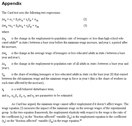
Since the gains from a $1.00 increase generally fall as income rises, and income shares are successively higher for each quintile, the gains relative to income share fall precipitously, from 5.8 in the lowest fifth to 0.3 for the wealthiest households. Thus, while arguably about 25% of the benefits from the increase miss their target (combining the top two fifths), the relative gains to those wealthier households are much smaller than those going to low-income households. The fact that the minimum wage is not tied to income, as is, for example, the EITC, means that it is not perfectly targeted-some of the gains from an increase actually go to high-earning families. But in terms of policy discussions, the minimum wage should not be judged solely on the basis of targeting because, as noted above, it is not merely an anti-poverty program. While it is partly intended to lift the incomes of low-income working families (regardless of their poverty status), it is also an important labor market institution, whose purpose is to set a floor on the low end of the labor market. In this regard, it serves to counterbalance the lack of bargaining power suffered by the economy’s lowest-paid workers (regardless of their income level). When the minimum wage is allowed to fall in real terms, it undermines this important labor market protection. Employment effects of minimum wage increases As mentioned before, one of the most commonly raised objections to increases in the minimum wage is that, by pricing some workers out of the labor market, the increase will hurt the very people it is intended to help. This question can be answered by looking at the empirical evidence, and, in this section, two sets of statistical tests are used to determine the job-loss effects of minimum wage increases. The first test, introduced by labor economist David Card (1992), exploits the variation between states to test the employment impact of the wage increase; the second test uses the changes in the minimum wage over time. THE CARD TEST Card’s (1992) test uses variation in state labor markets to measure the employment impact of the minimum wage. The Card test takes advantage of the fact that “[t]he imposition of a national minimum wage…provides a natural experiment in which the `treatment effect’ varies across states depending on the fraction of workers initially earning less than the new minimum” (1992, 22). The test essentially asks whether the pattern of employment changes across states is correlated with the share of workers in each state that were affected by the national increase. If the standard model of the labor market provides a good description of the low-wage labor market, employment losses should be greatest in states that initially had the highest shares of workers in the wage range affected by the minimum wage increase.[11] Card’s first analysis relied entirely on data from the CPS ORG but was later updated by Card and Krueger (1995) using a combination of CPS ORG data and published employment rates from the full monthly CPS. Our analysis follows Card and Krueger (1995) and uses both the CPS ORG (to define average wages and shares of workers that fall in specified wage ranges across the states) and the full monthly CPS (to provide the most accurate estimates of state employment variables). Updating the analysis in Card and Krueger (1995) for the 1996-97 increases required using data from October 1994 onward. This paper defines the wage for each individual in the underlying ORG sample as either his or her reported hourly wage, if the worker reports being an hourly-paid employee, or as the individual’s usual weekly earnings (which includes bonuses, tips, and commissions) divided by usual weekly hours worked.[12] This procedure is substantially similar to that used in Card (1992). The Card results: Tables 5 and 6 report results from the specification most in spirit with the original Card (1992) and Card and Krueger (1995) versions of the test (described by equations (2) and (3) in the appendix). All specifications use 1995 as the reference year. In both tables, columns (1) and (2) examine changes in state wages (Table 5) or state employment rates (Table 6) between 1995 and 1996, a period covering a full year after the first increase in the federal minimum wage.[13] Columns (3) and (4) examine changes between 1995 and 1997, a period covering two full years after the first increase and one full year after the second increase. Columns (5) and (6) examine changes between 1995 and 1998, a period covering three full years after the first increase and two full years after the second. Following Card (1992) and Card and Krueger (1995), the tables show the impact of the minimum wage on wages and employment with and without controlling for changes in the overall state employment rate for all men and women, ages 16-64. The top half of Table 5 reports the impact of changes in the federal minimum wage on the average state wage of teenagers. After controlling for changes in overall state employment (column 2), changes in average teen wages appear to be related (at the 5% level) to changes in the minimum wage. Average teen wages grew about 1.1% faster (coefficient of 0.11) for every 10 percentage points of the teen workforce in the range affected by the first increase. The initial impact of the full minimum wage increase was slightly larger, with a coefficient of 0.17 in column (4). Two years after the full increase (see column 6), the effect dipped slightly (coefficient of 0.15). The bottom half of Table 5 shows the results of similar regressions for adult workers with less than a high school degree. Across all three time periods, the impact of the minimum wage on average wages is large and statistically significant. As with teens, however, the effect of the minimum wage shows a mild inverted-U shape. The minimum wage effect rose from 0.29 in the first year after the first increase (see column 2) to 0.41 in the first ye
ar after the full increase (see column 4), only to fall to 0.33 after the second year of the full increase (see column 6).

Table 6 reports results from corresponding employment equations. As Card has argued, the minimum wage cannot affect employment if it doesn’t affect wages. For teens, the first increase led to a statistically significant decline in employment (column 2). The implied employment elasticity (the ratio of the fraction affected coefficient in Table 6 to the corresponding coefficient in Table 5) from this estimate is large, about -0.9. The employment impact, however, is smaller and not statistically significant for the full increase (see columns 4 and 6). The results for adults without a high school degree show that the first minimum wage increase had an economically large (elasticity of 0.5), statistically significant (at the 10% level), positive impact on less-educated workers. The positive employment effects of the initial increase, however, disappeared after the full increase was implemented (see columns 4 and 6). The estimates for 1995-97 and 1995-98 show small, statistically insignificant declines in employment for these workers.[14]

Table 7 applies two sets of specification tests to the employment regressions in Table 6. Following Card and Krueger, the first column shows the results of the estimated employment change across two years (1994 and 1995) in which no change in the minimum wage took place. If the Card test works well, then the minimum wage should have no effect on employment under these circumstances. In fact, the regressions give results that are close to zero (0.02 for teens, -0.01 for less-educated adults). The next three columns reproduce the employment regressions in Table 6, but use 1994 as the base year instead of 1995. Since the 1995 base year runs from October 1995 through September 1996, and since sometime during that period many employers probably became fairly certain that some form of minimum wage would be enacted,[15] some employers may have acted before the minimum wage went into effect by shedding workers, reducing hiring, or conceivably even raising wages. Wage and employment patterns from 1994, presumably, would be less likely to suffer from such contamination.[16] When 1994 is used as a base year instead of 1995, the minimum wage has no statistically significant impact on employment. The negative effect on teen employment of the first minimum wage increase (see Table 6, column 2) disappears with the change of base year, as does the corresponding positive employment effect for less-educated adults. The preceding regressions may also suffer from problems flowing from the choice of the control population. Some of the individuals in the experimental groups (16-19 year olds and 20-54 year olds with less than a high school education) are also members of the control population (the 16-64 year old population). The last three columns of Table 7 reproduce the main employment regressions from Table 6 but use the employment rate for 20-64 year olds with a high school degree or more as a control population. Eliminating the mechanical correlation between the control and the dependent variables reduces the strength of the relationship between the employment rates of the experimental population and that of the control group but has no meaningful impact on the estimated employment effects. Summarizing the Card results: The structure of the Card test and the availability of data through September 1999 allow separate analyses of impacts of the first, second, and full increases in the minimum wage over one- and two-year periods. Table 8 presents permutations of the estimated employment effects of the 1996-97 increases using 1994 and 1995 as the base year. The most striking feature of the table is the almost complete absence of employment effects on teens or less-than-high-school-educated adults from the full increase (see columns 5-8). The only statistically significant employment responses are confined to shorter-term tests of the individual increases.

For teens, the Card test shows some evidence of large employment losses (an elasticity of -1.0) in connection with the first increase (see column 1 in the top half of the table), but these losses are not robust when using 1994 as a base year. The test also shows strong employment gains (elasticities greater than 1.0) in both the first and second year after the second increase (see columns 3 and 4). The second increase, however, had no systematic impact on teen wages, weakening the case that the minimum wage change might have been responsible for the corresponding employment gains. For less-educated adults, the Card test shows large employment gains from the first increase (an elasticity of 0.6-see column 2, bottom half of table), but these gains are not robust when using 1994 as the base year. The test also found large employment losses in the first year after the second increase (an elasticity of -1.5 in column 3). The minimum wage increases, however, apparently had no systematic effect on the wages of less-educated adults over the same period, and, in any event, the job losses were no longer statistically significant a year later (see column 4).

TIME-SERIES MODEL While most of the recent work on the question of disemployment effects has been in the statistical framework presented above, the views of many economists and policy makers on the minimum wage were initially shaped by time-series analysis. This research is responsible for what was formerly the conventional wisdom: a 10% increase in the minimum wage will result in a 1-3% decline in the teenage employment rate. For older workers, the general thinking is that the elasticity is essentially zero. Though recent work, particularly that of Card and Krueger, has begun to erode the former consensus, the conventional wisdom is still held by many economists, as is evident in the results of a recent poll. This survey of labor economists, published in a journal of the American Economic Association (Fuchs et al. 1999), showed that, on average, the economists in this survey estimated that a 10% increase in the minimum wage would lower teenage employment 2.1%. This is right in the middle of the 1-3% range that has persisted since the time-series models were run in the early 1980s.[17] This view of the disemployment effects derives from reduced-form, time-series equations run by the Minimum Wage Study Commission back in the early 1980s (Brown et al. 1982). Their models regressed the log of teenage employment-to-population ratio on the logged Kaitz index (the minimum wage variable) and a set of controls. The Kaitz index is the minimum wage relative to the average non-supervisory worker wage, weighted by coverage and teenage employment, and summed over numerous industries. [18] Various analysts have pointed out limitations of this variable (see, for example, Card et al. 1994). Our use
of it here is not an endorsement; it is included out of an interest in trying to update the conventional wisdom, which was based on this variable. The controls in the original models were for the impact of the business cycle (captured through the unemployment rate of prime-age males), supply variables -such as the share of teenagers in the civilian population – and for seasonality (since teenage employment rates are highly seasonal). More recent work has extended the commission’s model by adding observations. Wellington (1991), and later Card and Krueger (1995), both show how the coefficient has become smaller in absolute value over time. Figure 5 makes this point by using the conventional time-series model to generate a set of coefficients on the Kaitz index when observations (quarters) are added one at a time starting in 1975 (what is known as a “rolling regression”). Note the upward drift of the estimate toward zero (left y-axis), along with the trend toward insignificance in the t-statistic as more observations (i.e., quarters) are added.[19] Such a pattern suggests that the minimum wage has a smaller disemployment effect over time. Since Wellington’s discovery that the disemployment effect was drifting toward zero, little analysis has been done to determine why this is the case. One possible explanation is that, as the minimum wage has fallen over time, and thus affected fewer workers, its “bite” has also fallen. A less binding minimum-one that was below the average market wage (the wage set by supply and demand in the labor market) for low-wage workers-would be expected to lead to fewer job-loss effects.[20] Another potential explanation for the trend in Figure 5 is that the low-wage workforce has become more productive over time, thus able to absorb minimum wage increases with less employment disruptions. (Hopefully future studies will look into these questions further.) The first row of Table 9 shows a series of regression coefficients on the minimum wage variable from different time-series approaches to the disemployment question. The first row shows that extending the basic model-the one that has shaped the conventional wisdom of a 1-3% disemployment effect noted above-through the first quarter of 2000 yields a statistically insignificant coefficient of -0.061. Thus, ignoring statistical significance, a 10% increase in the minimum wage would lower teenage employment by less than 1%. By this measure, the 1-3% job-loss consensus clearly needs updating.Since these basic time-series models were introduced into the debate, there have been significant strides in time-series analysis, particularly in the area of testing for stationarity, and paying closer attention to the evaluation and treatment of seasonality (as would be expected, teenage employment rates are highly seasonal in the U.S.).[21] To the extent that any of the variables in the time-series model are non-stationary (i.e., have unit roots), or the effect of seasonality is not fully extracted, the output from the traditional models is not reliable. More specifically, the results from such models are likely to find spuriously significant relationships. Paul Wolfson (1998) examines this issue and finds evidence of non-stationarity in some of the key variables and ineffective seasonal controls in the basic time-series models responsible for the 1-3% negative elasticity estimates. He suggests a model in which these variables are entered as first differences, and seasonality is controlled for by the addition of a lagged seasonal difference. Those estimates, shown in the bottom half of Table 9 (models 4 and 5), are consistently smaller than those in the basic quarterly model and are statistically insignificant. The model estimated in the second row replaces the quarterly dummies with seasonal adjusters for the log teenage employment rate from the U.S. Census seasonal adjustment procedure (X-12-ARIMA, which generates a different adjuster for each quarter).[22] While this procedure has the tendency of adding to the serial correlation in the residuals, various tests of the residuals from this regression showed them to be “white noise.”[23]

Nevertheless, running the model on seasonally adjusted data, as in model 2, engenders the possibility of various other econometric problems (Jaditz 1994). Thus, model 3 skirts the seasonality question by running the data on annual observations. While this obviously reduces the degrees of freedom (the model has 43 observations after adjusting the endpoints), the “nuisance parameters” can then be omitted from the quarterly models (the quarterly dummies, trends, and their interactions). The Kaitz coefficients in models 2 and 3 are less than half the magnitude of that of model 1, and are insignificant. Another way of getting around some of the unit root problems in the key variables is to model the non-stationary components using the structural model described in Harvey (1989). This approach has many advantages over the above models. First, such a model simultaneously controls for the non-stationarity of the dependent variable (log teen employment rates) without differencing while explicitly modelling the moving seasonality discussed above.[24]

The latter characteristic of teenage employment rates-moving seasonality-is shown in Figure 6, which plots each seasonal factor. As expected, teenage employment is highest in the summer months (Season 3) and lowest in Season 1 and Season 4. But note that the summer season’s effect drifts downward over time, from a high of about 0.18 log points in the mid-1960s to a low of about 0.10 at the end of the series. The Season 1 effect also becomes less negative over time. Together, these trends suggest that, while teenage employment rates remain highly seasonal, they are less so now than in the past. The structural model controls for this change in the regression. The coefficient on the log Kaitz index from the structural model, shown in Table 6, is -0.052, with a t-statistic of -1.62. The magnitude of the coefficient is between that of the basic model (1) and the basic model, differenced (4). The structural model seems to do a better job of both modeling moving seasonality (an advantage over model (1), which assigns some of the effect of seasonal variation to the minimum wage variable), and modeling the stochastic component of teenage employment rates (as opposed to the differencing approach used in (4), which tends to difference away too much of the relationship between the key variables). Summing up this econometric analysis, it should be noted that results from the Card tests suggest that the 1996-97 increases had no measurable effect on the employment opportunities of teenagers or adults without a high school degree. These tests shows no robust, statistically significant employment changes in response to the 1996-97 increases. Most estimates, especially those over the full set of increases, lie close to zero. In the case of teens, the Card test suggests employment fell in response to the first increase, but the estimate is sensitive to changing the base
year for the comparison and, in any event, is counteracted by slightly larger, statistically significant gains in employment associated with the second increase. The results for less-educated adults show the opposite pattern, with a marginally significant employment rise associated with the first increase and a significant decline associated with the second increase. Neither movement, however, is particularly robust, and estimates of the employment effects over the full increase are statistically insignificant and near zero in economic terms. Similarly, this update of the time-series analysis that originally shaped the conventional wisdom that minimum wage increases lead to job losses suggests that, were this analysis undertaken today, the results would be quite different. First, using variants of the original models run by the Minimum Wage Study Commission shows that the negative elasticity becomes smaller and less significant over time. Of equal importance are the advances in our understanding of this type of analysis, which suggest that these early models were incorrectly specified, leading to “false positives” (i.e., thinking that significant relationships have been identified where there are none). When these more recent methods are applied, the fragility of the relationship between the minimum wage (as measured by the Kaitz index) and teenage unemployment is evident. Conclusion Minimum wage increases have at least two purposes. The first is to lift the earnings of low-wage workers. Opponents of the policy have often raised the potential disemployment effects, but this analysis shows that minimum wage increases do not price low-wage workers out of the labor market. The employment effects, while negative in some models, never reach anywhere near the level where the benefits to low-wage workers would be outweighed by their costs in terms of job losses. These findings, especially when taking into consideration the characteristics and incomes of minimum wage workers and their families, provide convincing evidence that the policy is effective in raising the earnings of low-wage workers, most of whom (though not all) reside in below-average income households. The second purpose of the minimum wage is to maintain a floor underneath the low-wage labor market. This role of the minimum is important, because low-wage workers have historically had the least bargaining power in the U.S. workforce. As shown in Table 1, they are least likely to be represented by unions and more likely to be female or minority, two groups whose wages and incomes have historically been lowered by discrimination. Figure 3 makes the point that this floor used to be significantly higher, high enough, in fact, to lift a working mother with two children above the poverty line. This is no longer the case, and this worker must now depend on other supports, such as food stamps and the Earned Income Tax Credit, to provide her family with an income that enables the family to meet its basic needs. These subsidies are an important part of a package of income supports that help working families make ends meet. But it should also be stressed that the minimum wage, which has the direct effect of raising the market wage paid to the low-wage workforce, is an important component of that policy package.

The authors thank Paul Wolfson for helpful discussions and comments. Danielle Gao provided extensive research assistance. Abe Cambier helped with graphics. We thank the Annie E. Casey Foundation for support.

Endnotes 1. States can set their minimum wages above or below the federal level, and the higher of the two applies to covered workers (the vast majority of the low-wage workforce is covered by minimum wage under the Fair Labor Standards Act). Ten states and the District of Columbia have minimum wages that exceed that of the federal government: Alaska ($6.15), California ($5.75), Connecticut ($6.15), Delaware ($5.65), D.C. ($6.15), Hawaii ($5.25), Massachusetts ($6.00), Oregon ($6.50), Rhode Island ($5.65), Vermont ($5.75), and Washington ($6.50). 2. Throughout the study, we refer to those workers earning within a dollar of the minimum wage as minimum wage workers. More precisely, these are the workers who would be affected by a dollar increase in the minimum wage. 3. We deflate the minimum wage with the CPI-U-X1. This alternative deflator corrects the more commonly used CPI-U for the overstatement of price growth in that deflator over the late 1970s and early 1980s. 4. This wage series is derived from the CPS and is described in Mishel et al. (1999, Appendix B). 5. See endnote 1 for list of states with minimum wages higher than the federal level. For coverage criteria, see U.S. DOL (1998). 6. We can use the data in Table 1 to translate this increase into an annual aggregate amount, which comes to $7.4 billion. This amounts to 0.2% of the national wage bill of $4.5 trillion in 1999. 7. See Card and Krueger (1995, 160). 8. See Burkhauser (2000). 9. See Bernstein et al. (2000). 10. The hourly earnings of the quarter of the sample who are leaving the CPS rotation in March 1999 are used, since these respondents report the necessary information to derive this wage. The advantage of the March file in this context is that it also has family income and annual hours worked from the previous year (in this case 1998). We then identify those workers in March 1999 earning within $1.00 of the federal minimum wage that year (as in Table 1, making appropriate adjustments for states with higher minimums) and calculate the difference between their wage and $6.15. This difference is multiplied by their hours of work from the previous year to derive the yearly gains from a $1.00 increase. For example, if someone was earning $5.50 in March 1999, and worked 1,000 hours in 1998, there annual gain would be $650. Note that this method assumes no disemployment. We then sum the gains across each family, divide families into income fifths, and calculate the share of the annual gains going to each income fifth. The table also reports the income share and average income for each fifth.11. In the middle of a national economic boom, as was generally the case in 1996 and 1997, employment gains should be smallest in states with the highest share of workers in the affected range. 12. The wage data here are taken from CPS extracts created by the Economic Policy Institute and described in Mishel at al. (1999, Appendix B). 13. During the first 11-months of this year period, the federal minimum wage was $4.75; during the last month of this period the minimum wage was $5.15. 4. A separate analysis (not shown) applies five specification tests, from Card and Krueger (1995), to the regressions in Table 6. The tests don’t change the conclusions drawn from Table 6. 15. By May 1996, even some Republicans in Congress had proposed legislation to raise the minimum wage. 16. Few employers operating in the first year of the Republican-controlled 104th Congress would probably have expected a minimum wage increase in the second year of that Congress. 17. Interestingly, this same survey also provides some evidence that recent research, such as Card and Kreuger’s work, is weakening the disemployment consensus. The range of estimates from the survey shows that fully 30%
of the economists responded that an increase in the minimum wage would either raise teenage employment or leave it unchanged. The median estimate was a 1% decline, half the job loss predicted on average. The survey also asked economists to rate the desirability of the minimum wage increase on a scale from zero (“strongly oppose”) to 100 (“strongly favor”). The median estimate was 50, and the average estimate was 53. 18. See Bernstein and Schmitt (1998, appendix). 19. The coefficient is statistically insignificant when the “t-stat” line is above the straight line at -1.96 (t-statistics below this level in absolute value imply that the coefficient is not significantly distinguishable from zero, i.e., no disemployment effect). 20. Of course, the real market wage for low-wage workers has also fallen over time, but, as shown in Figure 2, not as quickly as the minimum. 21. A stationarity times series is (essentially) one in which the series has a constant mean and variance. 22. When the coefficient on the seasonal adjusters is close to one, as it is this regression, this reduces to running the model on a seasonally adjusted dependent variable. 23. Specifically, LM tests for correlation among the residuals at lags 2, 4, and 8 did not allow for rejection of the null hypothesis of no serial correlation in the residuals. 24. In the structural model, seasonality is modeled by comparing the teenage employment rate series to a series of trigonometric functions, with “peaks and valleys” at the season frequencies. To capture moving seasonality, the seasonal equation includes a disturbance term. The model also includes a stochastic trend and cycle component. Estimation was carried out using STAMP 6.0 software. 25. Neither Card (1992) nor Card and Krueger (1995) examined data for less-educated adults. 26. The elasticities reported in the preceding minimum wage analysis are employment elasticities with respect to increases in the federal minimum wage. The elasticities reported in the Card analysis are employment elasticities with respect to the actual wage changes induced by the minimum wage increases. References Bernstein, Jared, Chauna Brocht, and Maggie Spade-Aguilar. 2000. How Much Is Enough? Basic Family Budgets for Working Families. Washington, D.C.: Economic Policy Institute. Bernstein, Jared and John Schmitt. 1998. Making Work Pay: The Impact of the 1996-97 Minimum Wage Increase. Washington, D.C.: Economic Policy Institute. Card, David. 1992. “Using Regional Variation in Wages to Measure the Effects of the Federal Minimum Wage.” Industrial and Labor Relations Review. Vol. 46, No. 1, pp. 22-37. Card, David, and Alan Krueger. 1995. Myth and Measurement: The New Economics of the Minimum Wage. Princeton, N.J.: Princeton University Press. Fuchs, Victor R., Alan B. Krueger, and James M. Poterba. 1999.”Economists’ Views About Parameters, Values, and Policies: Survey Results in Labor and Public Economics.” The Journal of Economic Literature. Vol. 36, No. 3 (September), pp. 1387-1425. Harvey, Andrew C. 1989. Forecasting, Structural Time Series, and the Kalman Filter. Cambridge, Mass.: Cambridge University Press. Jaeger, David A. 1997. “Reconciling the Old and New Census Bureau Education Questions: Recommendations for Researchers.” Journal of Business & Economics Statistics. Vol. 15, No. 3, pp. 300-09. Mishel, Lawrence, Jared Bernstein, and John Schmitt. 2000. The State of Working America, 1998-99. Ithaca, N.Y.: Cornell University Press. Polivka, Anne E., and Stephen M. Miller. 1995. “The CPS After the Redesign: Refocusing the Economic Lens.” Bureau of Labor Statistics Research Paper. http://stats.bls.gov/orersrch/ec/ec950090.htm Schmitt, John. 2000. “Testing the Employment Impact of the 1996-97 Increases in the Federal Minimum Wage: Another Look at Card (1992) and Deere, Murphy, Welch (1995).” Economic Policy Institute, Washington, D.C. Unpublished paper. Webster, David. E. 1999. “Appendix B: Wage Analysis Computations,” in Mishel, et al. 2000. Wellington, Allison. 1991. “Effects of the Minimum Wage on the Employment Status of Youths: An Update.” Journal of Human Resources. Vol. 26, pp. 27-46. Wolfson, Paul. 1998. “A Reexamination of Time Series Evidence of the Effect of the Minimum Wage on Youth Employment and Unemployment.” University of Minnesota.