Executive summary
One common metric of monopsony power is the quit elasticity, measuring how much more likely a worker is to quit a job in response to a wage change. Experimental and quasi-experimental variation in wages across workers within a given job results in quit elasticities in the 2–3 range, implying that a 10% reduction in wages increases the probability of quitting by 20–30%. In a model with monopsonistic employers, a quit elasticity of 2–3 also implies that workers are paid about 80–85% of the value they produce. These results indicate that employer power is pervasive. We present observational evidence that historically disadvantaged groups have systematically lower quit elasticities, indicating they face even greater employer power. Because monopsony power comes from an inability of workers to voluntarily switch jobs, the quit rate and especially the quit elasticity can be a useful metric for judging the health of the labor market. Pervasive employer power alters the analysis of labor market policy in a number of important ways.
I. Introduction
Economists of all political stripes agree that a key restraint on employers in the labor market is the threat of workers quitting for other jobs. In theory, the voluntary flow of workers across firms, and in and out of the labor market, ensures that workers are rewarded according to “the law of one price,” which says that workers with similar characteristics, doing similar jobs, at similar firms, must be paid similar wages. Firms that attempt to underbid other firms should quickly lose all of their employees. Importantly, this logic applies to all attributes of a job, including nonwage benefits and working conditions more generally. When quitting is easy, no abusive bosses can last long, no predatory supervisors can keep their jobs, and other excessively onerous and unpleasant conditions of work will either be compensated for or competed away. Employers will bend over backward to provide amenities and wages to retain labor, and workers will be roughly indifferent across the jobs they can hope to get. As Milton Friedman wrote in Capitalism and Freedom (1962, 19), “the employee is protected from being coerced by his employer by the existence of other employers for whom he can work.”
The easy, and voluntary, flow of workers from job to job is one of the defining features of a competitive labor market. Competition, in turn, implies that firms cannot exercise power over their workers beyond what was agreed to in the employment contract, an assumption that is pervasive in economics, law, philosophy, and political science. The presumption that labor markets are defined by competition shapes both how we think about labor markets and how labor markets are governed both formally and informally. For example, the importance of an employee’s ability to quit is given great prominence in Epstein’s (1984, 947–8) well-known defense of the employee-at-will doctrine, which was clearly articulated in an oft-quoted passage from Payne v. Western & Atlantic Railroad, 81 Tenn. 518–19 (1884):
[M]en must be left, without interference to buy and sell where they please, and to discharge or retain employees at will for good cause or for no cause, or even for bad cause without thereby being guilty of an unlawful act per se. It is a right which an employee may exercise in the same way, to the same extent, for the same cause or want of cause as the employer.
In other words, the argument for at-will employment legislation, and much of existing employment law doctrine, rests on the presumption that both firms and workers can easily terminate an employment relationship. For workers, this presumption means that one can either easily transition to another, equally good job, or that unemployment is not penurious.
In reality, however, finding another job as good as the job one has is not so easy, and quitting a job is a fraught, complicated, and often costly decision. Jobs are complex, idiosyncratic relationships, and individuals value them for reasons that are often only theirs. A friendly coworker or generous boss, an easy commute, proximity to schools, and access to child or elder care all matter in the preferences a worker has for a job. Further, workers do not know about all the offers in the labor market: Most of us are not veteran job hunters, and we depend on a variety of ad hoc mechanisms and heuristics to find out about jobs that are good fits. The result is that job offers are rare, and even in tight labor markets finding a good new job depends a lot on luck in social networks, location, and skills.
The basic fact that work cannot be separated from workers means that limited mobility in response to wage differences across employers is pervasive, and this is true even without colluding or concentrated employers, noncompete agreements, or a variety of policies exacerbating this limitation. The availability of alternative offers, and so the cost of quitting a job, also likely varies by geography, race, and gender, as evidenced by, for example, persistently higher unemployment among Black men (Couch and Fairlie 2010) and the gendered expectations around female mobility.
When quitting a job is costly, employers have power over their employees—a form of power economists call monopsony power. This power allows firms to accept possibly higher turnover in exchange for paying workers lower wages, providing fewer benefits, and allowing worse working conditions, resulting in firms that are too small, pay too little, and have high turnover. This tradeoff is made possible by the fact that, when quitting is costly, workers are less willing to leave their jobs than they should be, and they are thus less sensitive to differences in wages and working conditions across various jobs. They leave jobs slowly, or not at all, thereby reducing the competitive pressure that firms may feel to eliminate discrepancies, and they are vulnerable to the arbitrary whims of their managers and employers.
Importantly, monopsony power does not require anticompetitive artifices such as noncompete agreements, collusion, or concentrated employers to generate employer market power. That is, monopsony power does not come solely from archetypically anticompetitive activities but rather is inherent to how laissez-faire labor markets work and how workers find and value jobs. As Alan Krueger noted in his Jackson Hole keynote address in 2018:
Although economists’ go-to model of the labor market is often one with perfect competition—where bargaining power is irrelevant because supply and demand determine the wage, and there is nothing firms can do about it—in many applications I think it is more appropriate to model the labor market as imperfectly competitive, subject to monopsony-like effects, collusive behavior by firms, search frictions, and surpluses that are bargained over. As a result of these labor market features, firms should be viewed as wage-setters or wage-negotiators, rather than wage-takers.1 (Krueger 2018, 267)
All monopsony requires is that quitting a job is costly, that these costs result in workers being so reluctant to leave their jobs that firms do not have to adjust wages or attributes of a job to keep workers, and that this cost differs from worker to worker in ways that employers may not be able to, or may choose not to, factor into their pay schemes.
An important by-product of monopsony power is that it gives employers latitude to use contractual devices like noncompete clauses to further lock in workers without having to compensate them for forgoing alternative employment (Starr, Prescott, and Bishara 2020). If the labor market were perfectly competitive, noncompete contracts would be perfectly offset by higher compensating wages (or other amenities)—a notion called a compensating wage differential—because workers would never accept the disamenity of forgoing future employment opportunities without being compensated by their current employer. When labor markets are monopsonistic, a noncompete contract will not necessarily be perfectly offset by higher wages, and so it might pay for an employer to use one. One could imagine an inverted-U relationship between noncompete contracts and the degree of monopsony. At one end, where the labor market is a perfect monopsony, there is no need for a noncompete agreement because there is only one employer and therefore nowhere else for workers to go; at the other end, where the labor market is perfectly competitive, there is no scope to introduce a noncompete agreement without losing all ability to recruit unless workers are sufficiently compensated, which would undermine the reason for using the agreement in the first place. But in between is a range of situations where workers may be willing to accept a noncompete agreement without demanding a commensurate increase in pay or benefits.
While noncompete clauses are one particularly important example, monopsony power means that, in general, the specific job and many of the features of a given employment relationship are designed to increase retention, particularly retention of high-productivity workers, potentially at the expense of less-productive workers in the same firm. This means that workplace cultures, tolerance of harassment, and even things like health benefit packages and workplace safety are not provided to satisfy the interest of the firm’s average workers but instead the most productive, or the ones most likely to quit. This potential for disparate treatment creates an important role for institutions of voice, such as collective bargaining, to represent the interests of all workers but most importantly those who are least likely to quit, because it is these workers over whom employers have the most power.
Although monopsony does not rely on the presence of anticompetitive practices like noncompete and antipoaching agreements and simple, naked collusion, anticompetitive practices certainly exacerbate monopsony. There is evidence that these practices are pervasive in today’s labor market (see Block and Harris 2021), and indeed even Adam Smith noted the predilection for employers to collude in setting wages. Yet merger screening policy overwhelmingly focuses on consumer welfare rather than worker welfare, despite the fact that mergers in thin labor markets have a detectable negative effect on wages (Arnold 2019; Prager and Schmitt 2019; Naidu, Posner, and Weyl 2018). New papers are coming out every few months that document negative effects of labor market concentration on wages, with the takeaway that roughly 10% higher concentration (as measured by the Herfindahl index) implies 0.1% to 1% lower wages.
One common method of measuring the degree of monopsony power—the method we use below—is the quit elasticity, a measure of how much more likely a worker is to quit a job in response to a (small) wage change. Monopsony comes, in part, from a reluctance of workers to quit their jobs. This implies a low quit elasticity because being reluctant to quit a job means that the likelihood an individual quits a job does not change very much in response to wage changes (i.e., a small decline in the wage does not increase the probability of quitting, and a small increase in the wage does not decrease the probability of quitting). Conversely, a competitive labor market implies a very high quit elasticity because even small changes in the wage should result in large-scale changes in quits.
Experimental and quasi-experimental variation in wages across workers within a given job results in quit elasticities in just the 2–3 range, implying that a 10% reduction in firm wages increases the probability that the average worker will quit by 20–30%. While this may seem like a lot, high competition theoretically implies the probability of quitting in response to even a small wage decrease should approach 100%. Moreover, trading off lower wages for somewhat higher turnover may be appealing to many firms, especially in situations where the cost of turnover is low. Evidence from survey data suggests quit elasticities that are even smaller, though these estimates are likely biased due to a failure to account for other labor market dynamics changing at the same time that may affect wages and the likelihood of quitting.
What is the cost to workers, and the profit to employers, of quit elasticities in such low ranges? And how might the impact vary between different groups of workers? Less is known on how the degree of monopsony power varies across historically disadvantaged groups, although related evidence on the comparative weakness of labor market outcomes experienced by these groups (Couch and Fairlie 2010) suggests that they should face higher levels of monopsony power as employers choose to leverage the weaker labor markets. Among our calculations (discussed in more detail below) are the following:
- If employers are strictly profit-maximizing, then a quit elasticity of 2–3 implies that workers are paid about 80–85% of the value they produce for the firm (i.e., marginal revenue product), with employers (or other input suppliers) pocketing the difference.
- Monopsony, as measured by lower quit elasticities, is higher in low-wage sectors such as retail and restaurants, for low-wage workers as measured by the bottom quartile of worker fixed-effects, and during business cycle downturns. These workers (and during these periods) may as a result reap an even lower share of their productivity.
- For men, however, the quit elasticity is 0.16 compared to 0.09 for women, implying that men are almost twice as likely to quit a job due to the same-size wage decline as are women.
- For white workers the quit elasticity is 0.12 compared to 0.07 for Black workers, implying that white workers are also almost twice as likely to quit a job in response to the same-size wage decline as are Black workers. Again, that historically disadvantaged groups—particularly Black workers, according to our results—are less sensitive to wage changes implies that firms have more leeway to actively reduce, or fail to increase, their pay because they are less likely to exercise the primary form of power available to them, which is to quit. And, while the elasticity estimates themselves are small compared to quasi-experimental evidence, the comparison of elasticities between groups is still a valid exercise.
Of course, no one would argue that labor markets are truly perfectly competitive, but viewed from this perspective, it is clear that elasticities of the size that have been estimated to date are far from what are expected in a competitive labor market. Even urban labor markets in low-wage, high-turnover sectors like food services or retail have low quit elasticities, despite being precisely the setting where labor markets ought to be competitive because there should be myriad alternative employment opportunities for workers and the workers ought to be easily substituted by firms.
The presence of monopsony suggests a more expanded view of how to judge the health of a labor market. Specifically, because monopsony power comes from an inability of workers to voluntarily switch jobs whenever they want, the voluntary job separation rate (or quit rate) can be a useful metric for judging the health of the economy, in addition to standard measures like the vacancy or unemployment rate. Its usefulness is partly because there is a “job ladder” that is an important source of wage growth during expansions and a major source of wage stagnation during downturns, when the ladder collapses; it is also partly because quits summarize the ability of workers to leave terrible working conditions that are not adequately compensated for. Further, the quit rate is a flow measure of labor market slackness, and so it moves more quickly than stock measures like unemployment, and relying on the former could speed up the timing of policy changes. Combined, these facets of the quit rate imply it should be a macroeconomic indicator that monetary and fiscal authorities pay attention to. If there is pervasive and persistent involuntary unemployment or underemployment, then there is always a “reserve army” of the unemployed available as new recruits, and so employers do not have to worry so much about preventing quits. Markets that do not guarantee full employment cannot guarantee worker freedom of choice or rely on worker exit to constrain employer exploitation.
One caveat to the literal monopsony interpretation of the labor market is that employers do not have to use all the monopsony power they have. For example, some firms may choose to use pay and/or benefits to elicit higher effort and quality or (even) stronger loyalty from their workers, steps that could in certain circumstances increase firm profitability.2 In order to deter shirking on the job, the threat of costly unemployment must be salient, and so monopsonists (particularly those without extensive workplace surveillance technologies) may have to pay wages higher than workers’ outside options. Incorporating effort implies that the output-reducing prediction of simple monopsony may not be borne out empirically, as powerful employers can impose faster work speed as well as lower wages. Similarly, employers can’t perfectly control their managers, and managerial interest in empire building may prevent employers from exercising all their monopsony power. Employers may also choose to set pay in a way that is largely unresponsive to local labor market conditions because, thanks to their power, they can be indifferent to the wage, paying arbitrary wages without worrying too much about losing all their workers. This indifference is revealed by the surprising degree of uniformity of wages paid by the same employer across disparate labor markets.3 Finally, some firms may choose to pay higher wages either in an attempt to increase their applicant pool and hopefully identify the most productive workers, or as an attempt to produce a reputation that consumers (or politicians) might reward.
II. Dynamic monopsony: The microeconomics of quits
Labor economists have long been divided over whether (and which) labor markets are best characterized by perfect competition or by monopsony. The defining feature of a perfectly competitive labor market is that a firm can hire as many workers as it desires at the prevailing wage rate, but also that it cannot hire any workers without paying that rate. Again, this implies that the firm faces an extremely elastic quit rate, or that decreasing wages even slightly below the market rate should result in essentially all of the workers quitting. The quintessential monopsony is a company town, where the only way a firm can hire more workers is to either draw in people already in the town but out of the labor force or draw new people into the town. In a monopsonistically competitive labor market there may be many employers, but it remains the case that, in order to recruit and retain more workers, firms must raise wages in order to overcome the costs workers incur in either entering the labor market or in switching jobs. The monopsony literature—and the term monopsony—dates back to 1933, when Joan Robinson published The Economics of Imperfect Competition (Robinson 1933). Since then, the literature on imperfect competition in labor markets has ballooned, not just in labor economics but also in law and economics, macroeconomics, international trade, and even industrial organization.4
Besides responding to outstanding puzzles in the minimum wage literature, the recent explosion of papers on monopsony reflects both the growing availability of detailed administrative data linking workers and employers and the decreasing cost of experimental interventions in real-world labor markets. Paradoxically, the decline of union coverage, minimum wages, and the willingness of firms to promote from within has made monopsony more visible. Recent empirical work suggests that a firm’s labor supply elasticity, which represents the combined impact of the change in workers quitting and the change in new employees when the wage changes, lies somewhere between 2 and 6, which implies that a 10% decrease in the wage decreases labor supply to the firm by 15–50%.
The sensitivity of firm-specific employment to wages, or the elasticity, is a direct measure of how much wage-setting power employers have. Set wages too low, and an employer will lose all its workers. Set wages too high, and an employer will lose profits. The just-right level of wages will trade off profit per worker with the number of workers staying at the firm. The more sensitive employment is to the wage—i.e., the larger the elasticity—the steeper this trade-off is, so that any attempt to lower worker wages will result in a much larger exodus of workers. In contrast, if this labor supply elasticity is low, then firms can pay workers low wages without having to worry about too many quitting. Variation in the elasticity a firm faces can come from differences in the type of work the firm requires, the location of the firm and the local labor market conditions the firm faces, and the pool of available labor from which the firm can hire.
Direct estimates of monopsony power that are obtained in thick labor markets—where there are both many workers and many employers—offer the most compelling evidence that monopsony is pervasive. Thick labor markets should mean that there are lots of workers looking for a job and lots of employer competition, and that no individual firm is large enough to be able to unilaterally alter conditions in the labor market; thus, labor supply elasticities to any one firm ought to be quite high. Generally, these estimates rely on the fact that a substantial fraction of people who quit employment at one firm become a new employee at another, meaning that there is a tight link between the average quit elasticity and the average labor supply elasticity to that firm. When the firm increases its wages, it both loses few workers and gains new workers, who will be quitting other firms.
Some of the most credible evidence on monopsony power in the United States is provided by the few randomized controlled experiments in which wages are randomized for identical jobs in markets with many wage-setters and little in the way of barriers to entry and movement between firms. Caldwell and Oehlsen (2018) randomized wages for Uber drivers, including those who also drove for Lyft. Examining the rate at which drivers switched between the two, they found a surprisingly low elasticity of between 4 and 5, suggesting that if the implied hourly wage was 10% higher at Uber (Lyft), then 40–50% of workers would switch to Lyft (Uber). Given that workers literally just have to switch apps on their phone, this is a surprisingly low rate of switching in response to a large wage difference. Dube, Jacobs, Naidu, and Suri (2020) experimentally varied wages for an identical task and found substantial monopsony power even on (putatively thick) Amazon Mechanical Turk.5 And, in a nonexperimental setting, Dube, Giuliano, and Leonard (2019), examining a large national retailer that implemented a national wage increase policy pretty much independently of any local labor market conditions, found that quits happened predominantly among those who didn’t get raises while their peers did. This paper illustrates both dimensions of monopsony: the constraints on internal wage differentiation and the extent of labor market competition. Workers quit a lot in response to arbitrary wage differences with their peers, but not so much in response to their own wages alone.6 A meta-analysis of the literature by Sokolova and Sorensen (2021) found an average labor supply elasticity of around 4, implying that a 10% increase in the wage is associated with a 40% increase in employment from a combination of fewer people leaving the firm and new people joining.
Other important evidence on labor supply elasticities comes from firm-specific shocks to labor productivity. In this literature, firms are suddenly hit with a shock that raises the productivity of labor (e.g., a patent is approved, a federal procurement bid is won, or student enrollment at a university goes up). If the employer has to raise or lower firm-specific wages, that suggests they have labor market power, and the resulting change in employment can be used to estimate labor supply elasticities. For example, Lamadon, Mogstad, and Setzler (2022) find a labor supply elasticity between 6 and 6.5 using shocks like this, while Goolsbee and Syverson (2019) find a labor supply elasticity of 1.9 (for full professors) to 7.8 (for assistant professors). One limitation of this literature is that firms can adjust many dimensions of compensation (e.g., hours) in response to productivity shocks (either upward or downward), making isolating the effect of wages difficult.
A. Monopsonistic competition: Evidence from matched worker firm data
In Bassier, Dube, and Naidu (2022), the quit elasticity is estimated by matching workers who are at the same firm and paid the same wage at time t–1 but leave to different firms at time t. They then look at how long workers stay at that next firm as a function of the wage change they got between t−1 and t. Workers lucky enough to land at a high-wage firm will stay longer before leaving again, and workers who land at a relatively low-wage firm will likely leave quickly.
This relationship is summarized in Figure A, reproduced from their paper. It shows a declining relationship, so that the probability of quitting decreases as the wage increases. Faster declines (a steeper slope) mean less monopsony power because workers are more sensitive to the wage change. The magnitude is similar to the other experimental and quasi-experimental estimates described above, where the quit elasticity was about 2 and implied a labor supply elasticity of around 4. So, if the employer decreases wages by 10%, the probability of quitting rises by 20%, it becomes 20% harder to get new recruits, and so overall labor supply to the firm falls by 40%. Quits matter, but they are hardly adequate as the sole device for restraining the capricious or exploitative whims of employers.
Quits as a function of firm wage policy
| Difference in firm component of log wage | Separations (relative to mean) | Polyfit |
|---|---|---|
| -0.1268 | 1.1176 | 1.1372 |
| -0.0707 | 1.1053 | 1.0822 |
| -0.0547 | 1.0847 | 1.0491 |
| -0.0437 | 1.0253 | 1.0233 |
| -0.0354 | 1.0313 | 1.0021 |
| -0.0285 | 0.9783 | 0.9836 |
| -0.0223 | 0.9685 | 0.9665 |
| -0.0169 | 0.9440 | 0.9513 |
| -0.0122 | 0.9413 | 0.9375 |
| -0.0079 | 0.9062 | 0.9251 |
| -0.0040 | 0.9153 | 0.9136 |
| -0.0005 | 0.8706 | 0.9028 |
| 0.0028 | 0.8898 | 0.8928 |
| 0.0060 | 0.8678 | 0.8834 |
| 0.0089 | 0.8765 | 0.8743 |
| 0.0118 | 0.8498 | 0.8657 |
| 0.0143 | 0.8323 | 0.8579 |
| 0.0167 | 0.8544 | 0.8506 |
| 0.0190 | 0.8334 | 0.8434 |
| 0.0211 | 0.8184 | 0.8368 |
| 0.0230 | 0.8177 | 0.8311 |
| 0.0248 | 0.8329 | 0.8255 |
| 0.0265 | 0.8289 | 0.8204 |
| 0.0279 | 0.8169 | 0.8159 |
| 0.0292 | 0.7972 | 0.8119 |
| 0.0303 | 0.8076 | 0.8087 |
| 0.0310 | 0.8014 | 0.8064 |
| 0.0317 | 0.8105 | 0.8043 |
| 0.0322 | 0.7948 | 0.8028 |
| 0.0324 | 0.8028 | 0.8020 |
| 0.0325 | 0.8050 | 0.8017 |
| 0.0326 | 0.8074 | 0.8014 |
| 0.0327 | 0.8047 | 0.8012 |
| 0.0328 | 0.8059 | 0.8009 |
| 0.0328 | 0.8730 | 0.8009 |
| 0.0329 | 0.7993 | 0.8005 |
| 0.0332 | 0.8018 | 0.7996 |
| 0.0336 | 0.8018 | 0.7984 |
| 0.0343 | 0.7839 | 0.7964 |
| 0.0351 | 0.7923 | 0.7940 |
| 0.0360 | 0.8104 | 0.7911 |
| 0.0371 | 0.7736 | 0.7877 |
| 0.0387 | 0.7716 | 0.7829 |
| 0.0405 | 0.7844 | 0.7774 |
| 0.0424 | 0.7490 | 0.7717 |
| 0.0443 | 0.7701 | 0.7659 |
| 0.0464 | 0.7684 | 0.7595 |
| 0.0489 | 0.7278 | 0.7523 |
| 0.0515 | 0.7283 | 0.7444 |
| 0.0544 | 0.7341 | 0.7359 |
| 0.0575 | 0.7241 | 0.7270 |
| 0.0607 | 0.7615 | 0.7176 |
| 0.0641 | 0.7230 | 0.7080 |
| 0.0678 | 0.7167 | 0.6977 |
| 0.0718 | 0.6921 | 0.6867 |
| 0.0763 | 0.6694 | 0.6744 |
| 0.0814 | 0.6507 | 0.6611 |
| 0.0871 | 0.6324 | 0.6466 |
| 0.0939 | 0.6196 | 0.6303 |
| 0.1016 | 0.6042 | 0.6129 |
| 0.1108 | 0.6095 | 0.5937 |
| 0.1233 | 0.5775 | 0.5712 |
| 0.1428 | 0.5564 | 0.5454 |
| 0.2223 | 0.5906 | 0.5971 |
Source: Authors’ analysis of Bassier, Dube, and Naidu, “Monoposony of Movers: The Elasticity of Labor Supply to Firm Wage Policies,” Working Paper no. 27755, National Bureau of Economic Research, 2022.
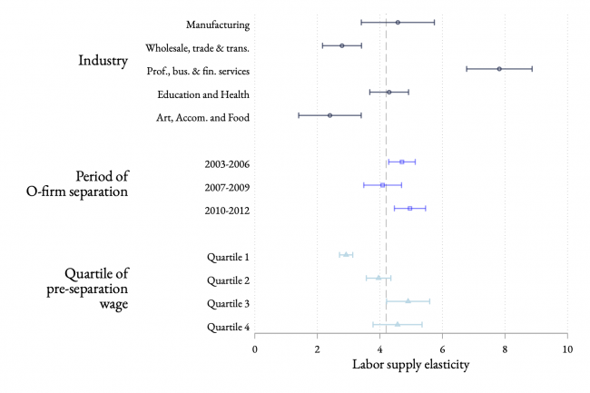
Further, the connection between aggregate labor market tightness and degree of employer power can be seen in differences in the labor supply elasticity across periods and across groups of workers (Figure B). Recessionary periods with higher unemployment have lower labor supply elasticities, implying more employer power, which makes sense because there are fewer alternative employment opportunities: fewer workers are quitting, and firms are hiring fewer workers. Low-wage workers have lower labor supply elasticities, implying that they face greater employer power. This is perhaps prima facie surprising because low-wage workers have higher turnover in general. But this turnover seems to be not particularly sensitive to the wage, and indeed one can imagine many competing risks, besides those that are wage-related, driving quit behavior for workers facing volatile schedules and other life shocks.
B. Heterogeneity: Evidence from the SIPP
The prospect of heterogeneity in monopsony power by gender dates to Joan Robinson’s early work on monopsony, which found women being paid less not because of lower productivity but because of social norms and intra-household bargaining power that dictated that wives move for their husbands and not vice versa. Employers, even nonsexist ones, would lower women’s wages relative to men’s, knowing that women’s outside options were circumscribed. A similar argument would apply to other ascriptive characteristics like race or even education: Employers are looking for “tags” for workers having better or worse outside options, and to the extent the law permits them to condition on those tags, they will. Even a nonracist employer would pay Black workers less, knowing that Black workers have both fewer other job options (as long as some racist employers exist in the same market) as well as lower average wealth and access to credit.7
We can explore worker-level heterogeneity a bit more in depth using the Survey of Income and Program Participation (SIPP).8 Here, we estimate the probability of voluntarily leaving one’s job for either another job or for nonemployment in each month for a given wage level in the previous month, while also adjusting both wages and the probability of quitting for human capital, demographic, and geographic factors.9 One issue to note is that both wages and the probability of quitting are, to some extent, affected by idiosyncratic worker-specific characteristics. That is, they are both endogenous, meaning that these estimates should not be taken as evidence that the causal effect of changes in the wage on the probability of quitting is different across groups, but rather that heterogeneity is present and worthy of future research. The following figures report the (residual) relative probability of quitting for each (residual) wage level, where wages are measured relative to the average (residual) wage in the group and the probability of quitting is measured relative to the probability of quitting for the middle-wage group. Residualizing wages and quits adjusts for differences in human capital and demographic characteristics, ensuring that comparisons are made among people with similar characteristics.10
Figures C–F show how the quit elasticity varies across the wage distribution (adjusted for covariates like education, age, geography) for all workers (Figure C) and by gender (Figure D), race/ethnicity (Figure E), and urban versus rural (Figure F). A comparison of slopes across groups gives an estimate of how monopsony power varies among them. Flatter slopes represent higher levels of monopsony power, because they imply that the probability of quitting is less sensitive to changes in the wage.
Quit rate as a function of the residual wage for all workers
| Everyone | |
|---|---|
| -1 | 0.200508 |
| -0.9 | 0.179179 |
| -0.8 | 0.185012 |
| -0.7 | 0.168296 |
| -0.6 | 0.13767 |
| -0.5 | 0.122989 |
| -0.4 | 0.09342 |
| -0.3 | 0.057343 |
| -0.2 | 0.037906 |
| -0.1 | 0.011954 |
| 0 | 0 |
| 0.1 | -0.01106 |
| 0.2 | -0.02715 |
| 0.3 | -0.01933 |
| 0.4 | -0.03426 |
| 0.5 | -0.01976 |
| 0.6 | -0.02593 |
| 0.7 | -0.02396 |
| 0.8 | -0.01699 |
| 0.9 | -0.02102 |
| 1 | 0.00724 |
Notes: Authors’ calculations using SIPP data from the 2004, 2008, and 2014 panels. Slope of each line for each group represents the quit elasticity, with steeper slopes representing a higher elasticity. Residual wage is the hourly wage adjusted for demographic characteristics, human capital, and survey year. The y-axis is the quit rate at each residual wage level relative to the quit rate at a residual wage of zero, or the average residual wage. Differences along axes are percent differences (e.g., a difference of 0.2 is a 20% difference).
Source: Authors’ analysis of Survey of Income and Program Participation (SIPP) data.
Quit rate as a function of the residual wage, by gender
| Men | Women | |
|---|---|---|
| -1 | 0.207644 | 0.163072 |
| -0.9 | 0.230153 | 0.155194 |
| -0.8 | 0.225035 | 0.148415 |
| -0.7 | 0.239974 | 0.138315 |
| -0.6 | 0.206351 | 0.119804 |
| -0.5 | 0.164454 | 0.082962 |
| -0.4 | 0.122331 | 0.078079 |
| -0.3 | 0.111737 | 0.046905 |
| -0.2 | 0.053268 | 0.028947 |
| -0.1 | 0.016935 | 0.018077 |
| 0 | 0 | 0 |
| 0.1 | -0.01768 | -0.00318 |
| 0.2 | -0.02599 | -0.00241 |
| 0.3 | -0.03634 | -0.01379 |
| 0.4 | -0.04614 | -0.00118 |
| 0.5 | -0.04797 | -0.00682 |
| 0.6 | -0.03457 | -0.0044 |
| 0.7 | -0.03519 | -0.00167 |
| 0.8 | -0.03888 | -0.00376 |
| 0.9 | -0.02095 | 0.010457 |
| 1 | -0.0405 | 0.016926 |
Notes: Authors’ calculations using SIPP data from the 2004, 2008, and 2014 panels. Slope of each line for each group represents the quit elasticity, with steeper slopes representing a higher elasticity. Residual wage is the hourly wage adjusted for demographic characteristics, human capital, and survey year. The y-axis is the quit rate at each residual wage level relative to the quit rate at a residual wage of zero, or the average residual wage. Differences along axes are percent differences (e.g., a difference of 0.2 is a 20% difference).
Source: Authors’ analysis of Survey of Income and Program Participation (SIPP) data.
Quit rate as a function of the residual wage, by race/ethnicity
| White | Black | Hispanic | |
|---|---|---|---|
| -1 | 0.189913 | 0.129485 | 0.298727 |
| -0.9 | 0.20256 | 0.128574 | 0.178887 |
| -0.8 | 0.194156 | 0.152753 | 0.218328 |
| -0.7 | 0.185029 | 0.069672 | 0.168559 |
| -0.6 | 0.161654 | 0.086714 | 0.144375 |
| -0.5 | 0.137933 | 0.069251 | 0.165405 |
| -0.4 | 0.100783 | 0.077699 | 0.103968 |
| -0.3 | 0.062151 | 0.038851 | 0.073941 |
| -0.2 | 0.04928 | 0.024295 | 0.07169 |
| -0.1 | 0.023869 | 0.020436 | 0.057355 |
| 0 | 0 | 0 | 0 |
| 0.1 | -0.00566 | -0.01357 | -0.02371 |
| 0.2 | -0.01005 | 0.010178 | -0.02934 |
| 0.3 | -0.02244 | -0.00376 | -0.0556 |
| 0.4 | -0.02062 | -0.00897 | -0.01524 |
| 0.5 | -0.0182 | -0.00325 | -0.06125 |
| 0.6 | -0.01961 | -0.0057 | -0.05534 |
| 0.7 | -0.00826 | -0.00263 | -0.02061 |
| 0.8 | -0.01689 | -0.01536 | -0.06262 |
| 0.9 | -0.01087 | -0.00762 | -0.08233 |
| 1 | 0.004361 | 0.074319 | 0.108596 |
Notes: Authors’ calculations using SIPP data from the 2004, 2008, and 2014 panels. Slope of each line for each group represents the quit elasticity, with steeper slopes representing a higher elasticity. Residual wage is the hourly wage adjusted for demographic characteristics, human capital, and survey year. The y-axis is the quit rate at each residual wage level relative to the quit rate at a residual wage of zero, or the average residual wage. Differences along axes are percent differences (e.g., a difference of 0.2 is a 20% difference).
Source: Authors’ analysis of Survey of Income and Program Participation (SIPP) data.
Quit rate as a function of the residual wage, by metropolitan status
| Rural | Urban | |
|---|---|---|
| -1 | 0.242015 | 0.154744 |
| -0.9 | 0.214808 | 0.173839 |
| -0.8 | 0.237972 | 0.182601 |
| -0.7 | 0.199639 | 0.168376 |
| -0.6 | 0.208436 | 0.133023 |
| -0.5 | 0.162001 | 0.103246 |
| -0.4 | 0.118284 | 0.08876 |
| -0.3 | 0.082979 | 0.053878 |
| -0.2 | 0.044969 | 0.035062 |
| -0.1 | 0.026689 | 0.016978 |
| 0 | 0 | 0 |
| 0.1 | 0.009394 | -0.00955 |
| 0.2 | -0.01874 | -0.02469 |
| 0.3 | -0.00688 | -0.01801 |
| 0.4 | -0.00467 | -0.03175 |
| 0.5 | -0.03483 | -0.02793 |
| 0.6 | -0.01028 | -0.01809 |
| 0.7 | -0.01025 | -0.02254 |
| 0.8 | -0.0191 | -0.01772 |
| 0.9 | 0.031924 | -0.01815 |
| 1 | 0.005069 | -0.00123 |
Notes: Authors’ calculations using SIPP data from the 2004, 2008, and 2014 panels. Slope of each line for each group represents the quit elasticity, with steeper slopes representing a higher elasticity. Residual wage is the hourly wage adjusted for demographic characteristics, human capital, and survey year. The y-axis is the quit rate at each residual wage level relative to the quit rate at a residual wage of zero, or the average residual wage. Differences along axes are percent differences (e.g., a difference of 0.2 is a 20% difference).
Source: Authors’ analysis of Survey of Income and Program Participation (SIPP) data.
The results are qualitatively similar to those seen in Figure A, though measured in different units. Specifically, the wage (horizontal) axis shows the percent difference between a given wage level and the average wage (which is defined as zero), and the quit rate (vertical) axis shows the percent difference in the probability of quitting between a given wage level and the average wage. Broadly, the quit elasticity tends to be smaller for low and high wages and larger for the middle of the wage distribution, as evidenced by the fact that the lines are largely horizontal in low (high) wages, indicating that the probability of quitting is similar across a wide range of wages (though much higher for low wages than for high wages). In the middle of the distribution monopsony power is lower, since this is the area where the probability of quitting declines as the wage increases. For example, Figure D shows that at a residual wage of -0.6 (an adjusted wage that is 60% below the average), the adjusted probability of quitting for men is about 20% higher than at the average wage (residual wage equals zero) but only 11% higher for women. Normalizing the adjusted probability of quitting to zero at the average wage for men and women shows that the probability of quitting falls faster for men as the wage increases in the bottom half of the wage distribution than it does for women. That is, for low-wage jobs an increase (decrease) in the wage decreases (increases) the probability of quitting more for men than it does for women. Similar patterns hold for Black versus white workers (Figure E) and urban versus rural workers (Figure F).
Figure G shows the quit elasticities implied by the slopes in Figures C–F, confirming that disadvantaged groups have lower quit elasticities and thus face more monopsony power. Variation across groups is meaningful and shows that employers have more power over those disadvantaged in the labor market (women, Blacks, and Hispanics). Overall, the implied quit elasticities in the SIPP—a 10% wage decrease resulting in a 1.2% increase in the probability of quitting (i.e., a quit elasticity of 0.12) are on the low end of the range seen in the literature using survey data. These are also very small relative to estimates identified using exogenous variation, but in any case nowhere close to the very high numbers (say 5 or higher) that perfect competition would imply. While the estimated quit elasticity is likely biased in this exercise, the estimates are meant to illustrate the differences across groups, as the wage variation here is clearly endogenous to many omitted factors, unlike the quasi-experimental estimates discussed above.
Overall quit elasticity by group
| Elasticity | |
|---|---|
| All | 0.1206 |
| Male | 0.1636 |
| Female | 0.0875 |
| Rural | 0.1395 |
| Urban | 0.1121 |
| White | 0.1243 |
| Black | 0.0660 |
| Hispanic | 0.1468 |
Notes: The quit elasticity is a linear approximation of the slope of the lines plotted in Figures D–F for each respective group.
Source: Authors’ analysis of Survey of Income and Program Participation (SIPP) data.
Men as a whole have the highest elasticity, with a 10% increase in the wage resulting in a 1.6% decrease in the probability of quitting, while Black individuals face the most monopsony power, with a 10% wage increase associated with a 0.7% decline in the probability of quitting. So, while elasticities are low for all groups, meaning employer power is pervasive, the results show employers have more power over disadvantaged groups in the labor market (women, Blacks, and Hispanics) than advantaged groups (whites and men). Again, the estimated elasticities are certainly biased toward zero due to important omitted variables that are correlated with both the wage and whether an individual quits a job, but we believe that comparisons across groups are still valid, at least for illustrative purposes.
C. Job ladders: The macroeconomics of quits
Recent research affirms the important role of quitting and labor market competition in driving wage growth. Traditionally, we measure the business cycle with unemployment, or the stock of workers out of a job who are actively looking for one. But this measure of the state of the labor market, while important, misses how tight labor markets help all workers by raising the degree of labor market competition. The job ladder (Moscarini and Postel-Vinay 2016), mentioned above, implies that during periods of expansion even employed workers get more and more offers for better jobs, leaving their employers no choice but to either raise wages or recruit new workers. At first employers recruit from the unemployed, and thus may not need to raise wages much, but once the pool of unemployed starts falling, employers begin poaching from each other, driving wage growth. Indeed, Moscarini and Postel-Vinay (2018) show that nominal wage growth responds to the quit rate even controlling for the unemployment rate, which supports the notion that the quit rate is an independent signal of a strong labor market along with the unemployment rate. A 1% decrease in the unemployment rate raises nominal wage growth by about 1 percentage point—the classic “wage curve” relationship between unemployment and wages. However, the authors also find that, even controlling for unemployment, a 1% increase in the employer-to-employer rate (i.e., leaving a job for another job, an admittedly imperfect proxy for quits) increases nominal hourly wage growth by 4 percentage points, and even more for people who actually switch jobs. The fall in the quit rate of roughly 0.5 over the Great Recession is thus associated with about a 2% fall in real wage growth. This pattern suggests that macroeconomic measurement may want to gauge tightness of the labor market based not just on the overall unemployment rate but also on the frequency of quits, in particular quits in response to wage differences across firms.
We have some spotty historical measures of quits, at least at an aggregate level, for manufacturing. Figure H shows the quit rate in manufacturing from two sources, the Historical Statistics of the United States (HSUS) and the Job Openings and Labor Turnover Survey (JOLTS), as well as the overall unemployment rate (from HSUS and the Bureau of Labor Statistics).11 If you want to see what a really tight labor market looks like, consider World Wars I and II, when the quit rate was the highest it has ever been, coincident with historically low unemployment rates. This pattern is consistent with the high pressure of the wartime economy and suggests that the labor market has never been as friendly to worker choice as it was then, even during the recent recovery.
Aggregate labor market tightness and quit rate over the 20th century
| year | Quits manufacturing (JOLTS) | Quits manufacturing (HSUS) | Unemployment rate |
|---|---|---|---|
| 1890 | 3.97 | ||
| 1891 | 4.49 | ||
| 1892 | 4.31 | ||
| 1893 | 6.77 | ||
| 1894 | 9.28 | ||
| 1895 | 8.48 | ||
| 1896 | 9.27 | ||
| 1897 | 8.51 | ||
| 1898 | 7.79 | ||
| 1899 | 5.85 | ||
| 1900 | 5.00 | ||
| 1901 | 4.14 | ||
| 1902 | 3.45 | ||
| 1903 | 3.53 | ||
| 1904 | 4.92 | ||
| 1905 | 3.89 | ||
| 1906 | 2.45 | ||
| 1907 | 3.07 | ||
| 1908 | 7.46 | ||
| 1909 | 5.65 | ||
| 1910 | 5.86 | ||
| 1911 | 7.02 | ||
| 1912 | 5.86 | ||
| 1913 | 5.74 | ||
| 1914 | 8.49 | ||
| 1915 | 9.04 | ||
| 1916 | 6.48 | ||
| 1917 | 5.18 | ||
| 1918 | 1.24 | ||
| 1919 | 5.8 | 2.34 | |
| 1920 | 8.4 | 5.16 | |
| 1921 | 2.2 | 11.33 | |
| 1922 | 4.2 | 8.56 | |
| 1923 | 6.2 | 4.32 | |
| 1924 | 2.7 | 5.29 | |
| 1925 | 3.1 | 4.68 | |
| 1926 | 2.9 | 2.90 | |
| 1927 | 2.1 | 3.90 | |
| 1928 | 2.2 | 4.74 | |
| 1929 | 2.7 | 2.89 | |
| 1930 | 1.9 | 8.94 | |
| 1931 | 1.1 | 15.65 | |
| 1932 | 0.9 | 22.89 | |
| 1933 | 1.1 | 20.9 | |
| 1934 | 1.1 | 16.2 | |
| 1935 | 1.1 | 14.39 | |
| 1936 | 1.3 | 9.97 | |
| 1937 | 1.5 | 9.18 | |
| 1938 | 0.8 | 12.47 | |
| 1939 | 1 | 11.27 | |
| 1940 | 1.1 | 9.51 | |
| 1941 | 2.4 | 5.99 | |
| 1942 | 4.6 | 3.10 | |
| 1943 | 6.3 | 1.77 | |
| 1944 | 6.2 | 1.23 | |
| 1945 | 6.1 | 1.93 | |
| 1946 | 5.2 | 3.95 | |
| 1947 | 4.1 | 4.41 | |
| 1948 | 3.4 | 3.73 | |
| 1949 | 1.9 | 5.92 | |
| 1950 | 2.3 | 5.13 | |
| 1951 | 2.9 | 2.73 | |
| 1952 | 2.8 | 2.89 | |
| 1953 | 2.8 | 3.57 | |
| 1954 | 1.4 | 6.77 | |
| 1955 | 1.9 | 5.22 | |
| 1956 | 1.9 | 4.15 | |
| 1957 | 1.6 | 4.61 | |
| 1958 | 1.1 | 7.13 | |
| 1959 | 1.5 | 5.88 | |
| 1960 | 1.3 | 5.51 | |
| 1961 | 1.2 | 6.49 | |
| 1962 | 1.4 | 5.93 | |
| 1963 | 1.4 | 5.99 | |
| 1964 | 1.5 | 5.18 | |
| 1965 | 1.9 | 4.66 | |
| 1966 | 2.6 | 3.65 | |
| 1967 | 2.3 | 3.30 | |
| 1968 | 2.5 | 3.24 | |
| 1969 | 2.7 | 2.79 | |
| 1970 | 2.1 | 4.18 | |
| 1971 | 1.8 | 5.92 | |
| 1972 | 2.3 | 5.63 | |
| 1973 | 2.8 | 4.87 | |
| 1974 | 2.4 | 5.49 | |
| 1975 | 1.4 | 8.98 | |
| 1976 | 1.7 | 8.27 | |
| 1977 | 1.8 | 7.2 | |
| 1978 | 2.1 | 5.44 | |
| 1979 | 2 | 5.03 | |
| 1980 | 1.5 | 6.77 | |
| 1981 | 1.3 | 7.61 | |
| 1982 | 9.93 | ||
| 1983 | 10.17 | ||
| 1984 | 7.99 | ||
| 1985 | 7.45 | ||
| 1986 | 7.00 | ||
| 1987 | 6.12 | ||
| 1988 | 5.37 | ||
| 1989 | 4.75 | ||
| 1990 | 5.51 | ||
| 1991 | 6.85 | ||
| 1992 | 7.49 | ||
| 1993 | 6.91 | ||
| 1994 | 6.10 | ||
| 1995 | 5.59 | ||
| 1996 | 5.41 | ||
| 1997 | 4.94 | ||
| 1998 | 4.50 | ||
| 1999 | 4.22 | ||
| 2000 | 1.90 | 3.97 | |
| 2001 | 1.24 | 4.74 | |
| 2002 | 1.23 | 5.78 | |
| 2003 | 1.18 | 5.99 | |
| 2004 | 1.30 | 5.54 | |
| 2005 | 1.36 | 5.08 | |
| 2006 | 1.44 | 4.61 | |
| 2007 | 1.47 | 4.62 | |
| 2008 | 1.16 | 5.80 | |
| 2009 | 0.72 | 9.28 | |
| 2010 | 0.81 | 9.61 | |
| 2011 | 0.90 | 8.93 | |
| 2012 | 0.90 | 8.08 | |
| 2013 | 0.93 | 7.36 | |
| 2014 | 0.98 | 6.16 | |
| 2015 | 1.08 | 5.28 | |
| 2016 | 1.20 | 4.88 | |
| 2017 | 1.53 | 4.34 | |
| 2018 | 1.64 | 3.89 | |
| 2019 | 1.61 | 3.67 | |
| 2020 | 1.30 | 8.65 |
Sources: Manufacturing quits from 1920 to 1980 and unemployment from 1890 to 1990 are from Historical Statistics of the United States (HSUS) Millennial Online Edition. Unemployment from 1990 forward are from the Bureau of Labor Statistics (BLS). Manufacturing quits from 2000 forward are from the Job Openings and Labor Turnover Survey (JOLTS).
Similarly, the lowest level of quits in manufacturing was observed during the historically highest rates of unemployment during the Great Depression. While we don’t have quit data for the late 19th century, the presence of substantial unemployment in the 20 years prior to World War I suggests that, even during the archetypical laissez-faire, freedom-of-contract period of Lochner, worker choice was circumscribed by labor market slack. Figure I, which shows the relationship between quits and the unemployment rate for the whole economy, not just manufacturing, confirms that quits rise substantially when unemployment drops or is low, and it shows that the positive correlation between quits and low unemployment remains true today. Times when most of the labor force has a job are also times when the employed have the most freedom to leave their jobs.
Employer-to-employer separations and unemployment rate as fraction of population
| Date | Employer-to-employer separations per worker, three-month average | Unemployment rate, three-month average |
|---|---|---|
| 1994-03-01 | 1.9 | 6.6% |
| 1994-04-01 | 1.7 | 6.5 |
| 1994-05-01 | 1.9 | 6.3 |
| 1994-06-01 | 1.9 | 6.2 |
| 1994-07-01 | 2.0 | 6.1 |
| 1994-08-01 | 2.1 | 6.1 |
| 1994-09-01 | 2.1 | 6.0 |
| 1994-10-01 | 1.9 | 5.9 |
| 1994-11-01 | 1.5 | 5.8 |
| 1994-12-01 | 1.5 | 5.6 |
| 1995-01-01 | 1.6 | 5.6 |
| 1995-02-01 | 1.6 | 5.5 |
| 1995-03-01 | 1.6 | 5.5 |
| 1995-04-01 | 1.5 | 5.5 |
| 1995-09-01 | 1.6 | 5.6 |
| 1995-10-01 | 1.8 | 5.6 |
| 1995-11-01 | 1.7 | 5.6 |
| 1995-12-01 | 1.6 | 5.6 |
| 1996-01-01 | 1.5 | 5.6 |
| 1996-02-01 | 1.6 | 5.6 |
| 1996-03-01 | 1.5 | 5.5 |
| 1996-04-01 | 1.6 | 5.5 |
| 1996-05-01 | 1.6 | 5.6 |
| 1996-06-01 | 1.8 | 5.5 |
| 1996-07-01 | 1.9 | 5.5 |
| 1996-08-01 | 1.9 | 5.3 |
| 1996-09-01 | 1.9 | 5.3 |
| 1996-10-01 | 1.8 | 5.2 |
| 1996-11-01 | 1.5 | 5.3 |
| 1996-12-01 | 1.5 | 5.3 |
| 1997-01-01 | 1.5 | 5.4 |
| 1997-02-01 | 1.6 | 5.3 |
| 1997-03-01 | 1.5 | 5.2 |
| 1997-04-01 | 1.5 | 5.2 |
| 1997-05-01 | 1.6 | 5.1 |
| 1997-06-01 | 1.7 | 5.0 |
| 1997-07-01 | 1.8 | 4.9 |
| 1997-08-01 | 1.9 | 4.9 |
| 1997-09-01 | 1.9 | 4.9 |
| 1997-10-01 | 1.8 | 4.8 |
| 1997-11-01 | 1.7 | 4.7 |
| 1997-12-01 | 1.5 | 4.7 |
| 1998-01-01 | 1.5 | 4.6 |
| 1998-02-01 | 1.6 | 4.6 |
| 1998-03-01 | 1.6 | 4.6 |
| 1998-04-01 | 1.6 | 4.5 |
| 1998-05-01 | 1.7 | 4.5 |
| 1998-06-01 | 1.8 | 4.4 |
| 1998-07-01 | 1.9 | 4.5 |
| 1998-08-01 | 1.9 | 4.5 |
| 1998-09-01 | 1.9 | 4.5 |
| 1998-10-01 | 1.8 | 4.5 |
| 1998-11-01 | 1.6 | 4.5 |
| 1998-12-01 | 1.5 | 4.4 |
| 1999-01-01 | 1.5 | 4.4 |
| 1999-02-01 | 1.5 | 4.4 |
| 1999-03-01 | 1.6 | 4.3 |
| 1999-04-01 | 1.6 | 4.3 |
| 1999-05-01 | 1.7 | 4.2 |
| 1999-06-01 | 1.7 | 4.3 |
| 1999-07-01 | 1.8 | 4.3 |
| 1999-08-01 | 2.0 | 4.3 |
| 1999-09-01 | 2.0 | 4.2 |
| 1999-10-01 | 1.9 | 4.2 |
| 1999-11-01 | 1.7 | 4.1 |
| 1999-12-01 | 1.6 | 4.1 |
| 2000-01-01 | 1.6 | 4.0 |
| 2000-02-01 | 1.7 | 4.0 |
| 2000-03-01 | 1.7 | 4.0 |
| 2000-04-01 | 1.7 | 4.0 |
| 2000-05-01 | 1.8 | 3.9 |
| 2000-06-01 | 1.9 | 3.9 |
| 2000-07-01 | 1.9 | 4.0 |
| 2000-08-01 | 2.0 | 4.0 |
| 2000-09-01 | 2.0 | 4.0 |
| 2000-10-01 | 2.0 | 4.0 |
| 2000-11-01 | 1.6 | 3.9 |
| 2000-12-01 | 1.6 | 3.9 |
| 2001-01-01 | 1.6 | 4.0 |
| 2001-02-01 | 1.7 | 4.1 |
| 2001-03-01 | 1.6 | 4.2 |
| 2001-04-01 | 1.4 | 4.3 |
| 2001-05-01 | 1.5 | 4.3 |
| 2001-06-01 | 1.6 | 4.4 |
| 2001-07-01 | 1.9 | 4.5 |
| 2001-08-01 | 1.9 | 4.7 |
| 2001-09-01 | 1.8 | 4.8 |
| 2001-10-01 | 1.6 | 5.1 |
| 2001-11-01 | 1.4 | 5.3 |
| 2001-12-01 | 1.4 | 5.5 |
| 2002-01-01 | 1.4 | 5.6 |
| 2002-02-01 | 1.4 | 5.7 |
| 2002-03-01 | 1.4 | 5.7 |
| 2002-04-01 | 1.4 | 5.8 |
| 2002-05-01 | 1.4 | 5.8 |
| 2002-06-01 | 1.6 | 5.8 |
| 2002-07-01 | 1.6 | 5.8 |
| 2002-08-01 | 1.7 | 5.8 |
| 2002-09-01 | 1.6 | 5.7 |
| 2002-10-01 | 1.5 | 5.7 |
| 2002-11-01 | 1.3 | 5.8 |
| 2002-12-01 | 1.3 | 5.9 |
| 2003-01-01 | 1.2 | 5.9 |
| 2003-02-01 | 1.3 | 5.9 |
| 2003-03-01 | 1.2 | 5.9 |
| 2003-04-01 | 1.2 | 5.9 |
| 2003-05-01 | 1.3 | 6.0 |
| 2003-06-01 | 1.4 | 6.1 |
| 2003-07-01 | 1.5 | 6.2 |
| 2003-08-01 | 1.5 | 6.2 |
| 2003-09-01 | 1.5 | 6.1 |
| 2003-10-01 | 1.4 | 6.1 |
| 2003-11-01 | 1.2 | 6.0 |
| 2003-12-01 | 1.1 | 5.8 |
| 2004-01-01 | 1.2 | 5.7 |
| 2004-02-01 | 1.3 | 5.7 |
| 2004-03-01 | 1.3 | 5.7 |
| 2004-04-01 | 1.3 | 5.7 |
| 2004-05-01 | 1.4 | 5.7 |
| 2004-06-01 | 1.4 | 5.6 |
| 2004-07-01 | 1.5 | 5.6 |
| 2004-08-01 | 1.6 | 5.5 |
| 2004-09-01 | 1.6 | 5.4 |
| 2004-10-01 | 1.5 | 5.4 |
| 2004-11-01 | 1.4 | 5.4 |
| 2004-12-01 | 1.3 | 5.4 |
| 2005-01-01 | 1.3 | 5.4 |
| 2005-02-01 | 1.3 | 5.4 |
| 2005-03-01 | 1.4 | 5.3 |
| 2005-04-01 | 1.3 | 5.3 |
| 2005-05-01 | 1.4 | 5.2 |
| 2005-06-01 | 1.5 | 5.1 |
| 2005-07-01 | 1.5 | 5.0 |
| 2005-08-01 | 1.6 | 5.0 |
| 2005-09-01 | 1.6 | 5.0 |
| 2005-10-01 | 1.5 | 5.0 |
| 2005-11-01 | 1.3 | 5.0 |
| 2005-12-01 | 1.2 | 5.0 |
| 2006-01-01 | 1.3 | 4.9 |
| 2006-02-01 | 1.4 | 4.8 |
| 2006-03-01 | 1.3 | 4.7 |
| 2006-04-01 | 1.3 | 4.7 |
| 2006-05-01 | 1.4 | 4.7 |
| 2006-06-01 | 1.5 | 4.6 |
| 2006-07-01 | 1.6 | 4.6 |
| 2006-08-01 | 1.6 | 4.7 |
| 2006-09-01 | 1.6 | 4.6 |
| 2006-10-01 | 1.5 | 4.5 |
| 2006-11-01 | 1.3 | 4.5 |
| 2006-12-01 | 1.3 | 4.4 |
| 2007-01-01 | 1.2 | 4.5 |
| 2007-02-01 | 1.2 | 4.5 |
| 2007-03-01 | 1.2 | 4.5 |
| 2007-04-01 | 1.1 | 4.5 |
| 2007-05-01 | 1.2 | 4.4 |
| 2007-06-01 | 1.3 | 4.5 |
| 2007-07-01 | 1.4 | 4.6 |
| 2007-08-01 | 1.3 | 4.6 |
| 2007-09-01 | 1.3 | 4.7 |
| 2007-10-01 | 1.3 | 4.7 |
| 2007-11-01 | 1.2 | 4.7 |
| 2007-12-01 | 1.1 | 4.8 |
| 2008-01-01 | 1.1 | 4.9 |
| 2008-02-01 | 1.1 | 5.0 |
| 2008-03-01 | 1.1 | 5.0 |
| 2008-04-01 | 1.1 | 5.0 |
| 2008-05-01 | 1.1 | 5.2 |
| 2008-06-01 | 1.2 | 5.3 |
| 2008-07-01 | 1.2 | 5.6 |
| 2008-08-01 | 1.2 | 5.8 |
| 2008-09-01 | 1.2 | 6.0 |
| 2008-10-01 | 1.1 | 6.2 |
| 2008-11-01 | 1.0 | 6.5 |
| 2008-12-01 | 0.9 | 6.9 |
| 2009-01-01 | 0.9 | 7.3 |
| 2009-02-01 | 0.9 | 7.8 |
| 2009-03-01 | 0.9 | 8.3 |
| 2009-04-01 | 0.9 | 8.7 |
| 2009-05-01 | 1.0 | 9.0 |
| 2009-06-01 | 1.0 | 9.3 |
| 2009-07-01 | 0.9 | 9.5 |
| 2009-08-01 | 0.9 | 9.5 |
| 2009-09-01 | 0.9 | 9.6 |
| 2009-10-01 | 0.9 | 9.8 |
| 2009-11-01 | 0.8 | 9.9 |
| 2009-12-01 | 0.8 | 9.9 |
| 2010-01-01 | 0.9 | 9.9 |
| 2010-02-01 | 0.9 | 9.8 |
| 2010-03-01 | 0.9 | 9.8 |
| 2010-04-01 | 0.9 | 9.9 |
| 2010-05-01 | 0.8 | 9.8 |
| 2010-06-01 | 0.9 | 9.6 |
| 2010-07-01 | 1.0 | 9.5 |
| 2010-08-01 | 1.1 | 9.4 |
| 2010-09-01 | 1.0 | 9.5 |
| 2010-10-01 | 0.9 | 9.5 |
| 2010-11-01 | 0.8 | 9.6 |
| 2010-12-01 | 0.8 | 9.5 |
| 2011-01-01 | 0.8 | 9.4 |
| 2011-02-01 | 0.9 | 9.1 |
| 2011-03-01 | 0.9 | 9.0 |
| 2011-04-01 | 0.9 | 9.0 |
| 2011-05-01 | 0.9 | 9.0 |
| 2011-06-01 | 0.9 | 9.1 |
| 2011-07-01 | 1.0 | 9.0 |
| 2011-08-01 | 1.0 | 9.0 |
| 2011-09-01 | 1.0 | 9.0 |
| 2011-10-01 | 1.0 | 8.9 |
| 2011-11-01 | 0.8 | 8.8 |
| 2011-12-01 | 0.9 | 8.6 |
| 2012-01-01 | 0.9 | 8.5 |
| 2012-02-01 | 0.9 | 8.4 |
| 2012-03-01 | 0.9 | 8.3 |
| 2012-04-01 | 0.8 | 8.2 |
| 2012-05-01 | 0.9 | 8.2 |
| 2012-06-01 | 0.9 | 8.2 |
| 2012-07-01 | 1.0 | 8.2 |
| 2012-08-01 | 1.0 | 8.2 |
| 2012-09-01 | 1.0 | 8.0 |
| 2012-10-01 | 0.9 | 7.9 |
| 2012-11-01 | 0.9 | 7.8 |
| 2012-12-01 | 0.9 | 7.8 |
| 2013-01-01 | 0.9 | 7.9 |
| 2013-02-01 | 0.9 | 7.9 |
| 2013-03-01 | 0.9 | 7.7 |
| 2013-04-01 | 0.9 | 7.6 |
| 2013-05-01 | 0.9 | 7.5 |
| 2013-06-01 | 0.9 | 7.5 |
| 2013-07-01 | 1.0 | 7.4 |
| 2013-08-01 | 1.0 | 7.3 |
| 2013-09-01 | 1.0 | 7.2 |
| 2013-10-01 | 1.0 | 7.2 |
| 2013-11-01 | 0.9 | 7.1 |
| 2013-12-01 | 0.9 | 6.9 |
| 2014-01-01 | 0.9 | 6.7 |
| 2014-02-01 | 1.0 | 6.7 |
| 2014-03-01 | 0.9 | 6.7 |
| 2014-04-01 | 0.9 | 6.5 |
| 2014-05-01 | 1.0 | 6.4 |
| 2014-06-01 | 1.0 | 6.2 |
| 2014-07-01 | 1.1 | 6.2 |
| 2014-08-01 | 1.1 | 6.1 |
| 2014-09-01 | 1.1 | 6.1 |
| 2014-10-01 | 1.0 | 5.9 |
| 2014-11-01 | 0.9 | 5.8 |
| 2014-12-01 | 0.9 | 5.7 |
| 2015-01-01 | 0.9 | 5.7 |
| 2015-02-01 | 1.0 | 5.6 |
| 2015-03-01 | 1.0 | 5.5 |
| 2015-04-01 | 1.0 | 5.4 |
| 2015-05-01 | 0.9 | 5.5 |
| 2015-06-01 | 1.0 | 5.4 |
| 2015-07-01 | 1.1 | 5.4 |
| 2015-08-01 | 1.1 | 5.2 |
| 2015-09-01 | 1.1 | 5.1 |
| 2015-10-01 | 1.1 | 5.0 |
| 2015-11-01 | 1.0 | 5.0 |
| 2015-12-01 | 1.0 | 5.0 |
| 2016-01-01 | 1.0 | 5.0 |
| 2016-02-01 | 1.0 | 4.9 |
| 2016-03-01 | 0.9 | 4.9 |
| 2016-04-01 | 0.9 | 5.0 |
| 2016-05-01 | 1.0 | 4.9 |
| 2016-06-01 | 1.1 | 4.9 |
| 2016-07-01 | 1.1 | 4.8 |
| 2016-08-01 | 1.2 | 4.9 |
| 2016-09-01 | 1.2 | 4.9 |
| 2016-10-01 | 1.1 | 4.9 |
| 2016-11-01 | 1.0 | 4.9 |
| 2016-12-01 | 0.9 | 4.8 |
| 2017-01-01 | 0.9 | 4.7 |
| 2017-02-01 | 1.0 | 4.7 |
| 2017-03-01 | 1.0 | 4.6 |
| 2017-04-01 | 1.0 | 4.5 |
| 2017-05-01 | 1.0 | 4.4 |
| 2017-06-01 | 1.0 | 4.4 |
| 2017-07-01 | 1.1 | 4.3 |
| 2017-08-01 | 1.2 | 4.3 |
| 2017-09-01 | 1.1 | 4.3 |
| 2017-10-01 | 1.1 | 4.2 |
| 2017-11-01 | 0.9 | 4.2 |
| 2017-12-01 | 0.9 | 4.1 |
| 2018-01-01 | 1.0 | 4.1 |
| 2018-02-01 | 1.0 | 4.1 |
| 2018-03-01 | 0.9 | 4.1 |
| 2018-04-01 | 0.9 | 4.0 |
| 2018-05-01 | 0.9 | 3.9 |
| 2018-06-01 | 1.0 | 3.9 |
| 2018-07-01 | 1.1 | 3.9 |
| 2018-08-01 | 1.1 | 3.9 |
| 2018-09-01 | 1.1 | 3.8 |
| 2018-10-01 | 1.0 | 3.8 |
| 2018-11-01 | 0.9 | 3.7 |
| 2018-12-01 | 0.9 | 3.8 |
| 2019-01-01 | 1.0 | 3.9 |
| 2019-02-01 | 1.0 | 3.9 |
| 2019-03-01 | 1.0 | 3.9 |
| 2019-04-01 | 0.9 | 3.7 |
| 2019-05-01 | 0.9 | 3.7 |
| 2019-06-01 | 1.0 | 3.6 |
| 2019-07-01 | 1.1 | 3.7 |
| 2019-08-01 | 1.1 | 3.7 |
Source: Authors’ analysis of Federal Reserve Board data.
However, the very fact of cyclicality suggests that the market does not reliably deliver freedom in the workplace. The business cycle is as capricious as and less accountable than any monarch. If quitting is the primary force that disciplines employer behavior, then the cyclicality of quits suggests that employers are not always tightly constrained by market forces. In fact, employers are rarely constrained by market forces as the economy is rarely in periods of sustained low unemployment. As long as there is structural involuntary unemployment, employers will have the whip hand in setting wages and working conditions. The very fact of booms and busts tracking the quitting behavior of workers suggests that the real freedom experienced by workers, measured by the job options available rather than the current job, is higher when the economy is running hot, and choices are dramatically limited when unemployment is high. This is particularly true for historically disadvantaged groups and now generally true for less-educated workers, because of both the persistently higher rates of unemployment faced by these workers and the higher cyclicality in employment among these groups (particularly for men).
Some evidence on the sources of differential Black unemployment is provided in Couch and Fairlie (2010), who looked at matched Current Population Survey data on transitions from unemployment (and nonparticipation) for Black and white workers. They found that the gap in racial unemployment rates is highest at the lows of the business cycle and that little of this is explained by standard human capital variables like education and age. Thus, tight labor markets likely play an important role in mitigating racial inequality.
One practical way to implement these labor market proxies for economic freedom into macroeconomic policymaking is to use the quit rate for marginalized groups to augment measures of labor market slack, as mentioned above. Full employment becomes measured not just by the number of people looking for work who are unable to get it, but also by the real freedoms experienced by workers with jobs, proxied by their readiness to exercise exit.
One disadvantage of this measure is that the raw quit rate alone doesn’t distinguish between workers who don’t quit because they have a great job and those who don’t quit because they have terrible outside options. For example, Reich and Prins (2020), using data from the National Longitudinal Survey of Youth, show that prior incarceration reduces the responsiveness of quitting to job satisfaction. While people with prior incarceration are more likely to quit in absolute terms as their jobs worsen or options improve, their response has less to do with job conditions than it does for individuals without any experience of incarceration. For reasons such as this, raw quit rates should be supplemented by estimates of the quit elasticity, which manipulate the quality of the job or the outside options and measure the quit response.
But on average, the job ladder/dynamic monopsony model implies that increases in the quit rate are also likely to track the quit elasticity. Just by the fact that quits are most common at low-wage jobs and much rarer at high-wage jobs, the average level of quits is likely, in practice, to be correlated with the elasticity of labor supply facing the firm: when quits are common, the gap in quits between high- and low-wage firms is much higher, so the elasticity is higher. This is consistent with the procyclicality of the quit elasticity measured above. Why? Because if you’re at a firm that pays a very high wage for a given job, you aren’t likely to quit, because there aren’t many offers that are better than the job you have. So, the bulk of quitting is happening for workers at lower wages. Since the number of quits at the top of the labor market is small and pretty constant, the business-cycle quit variation is likely driven by workers leaving low-wage firms, and so the difference in quits between low-wage and high-wage firms, i.e., the sensitivity of quits to wage differences, is highest when the overall quit rate is high.
Some preliminary evidence suggests that this combination of high tightness with high unemployment happened during the post-COVID-19 Great Resignation, in which quits were high, the quit elasticity was high,12 and real wages were growing at the bottom of the distribution, even as unemployment was elevated (if declining).
D. Implications of real-world quit elasticities and employer power
There is a long history of the presumption of competitiveness in labor markets being used to weaken legal protections for workers. Bagenstos (2020) presents evidence that the presumption of no employer power is still pervasive in the law and has the adverse impact of undercutting the constitutional, statutory, and common law basis of workplace protections. Specifically, he examines the Lochner-era freedom-of-contract assumptions being used to justify at-will employment, forced arbitration, and limited enforcement of health and safety regulation. Essentially, almost any employment condition that a worker will accept is presumed to be the outcome of competition in the labor market, where contracts offered by employers can readily be turned down by workers. This presumption was illustrated in the U.S. Supreme Court’s recent decision on forced arbitration in Epic Systems Corp. v. Lewis, 138 S. Ct. 1612 (2018), in which the majority opinion, written by Justice Gorsuch, invokes freedom of contract in the first sentence. Were the forced arbitration agreements genuinely bilateral? Petitioner Epic Systems e-mailed its employees an arbitration agreement requiring resolution of wage and hours claims by individual arbitration. If the employees “continue[d] to work at Epic,” they would be “deemed to have accepted th[e] Agreement” (at 1649). The underlying presumption was that workers could readily quit to another job as good as the one they had at Epic. The dissent by Justice Ginsburg focused on the employer-employee power imbalance: “To explain why the Court’s decision is egregiously wrong, I first refer to the extreme imbalance once prevalent in our Nation’s workplaces, and Congress’ aim in the NLGA [Norris-LaGuardia Act] and the NLRA [National Labor Relations Act] to place employers and employees on a more equal footing” (at 1633).
The opinion in 1905’s Lochner v. New York, 198 U.S. 45 (1905), held that “the freedom of master and employee to contract with each other in relation to their employment, and in defining the same, cannot be prohibited or interfered with, without violating the Federal Constitution” (at 64). In a nutshell, the argument held that, since there was no externality or social problem (in the baking industry), there was no need for the state to use its police power to regulate labor markets. Until weakened by the New Deal, Lochner held considerable sway in preempting labor market regulation.
One could imagine the justification of Lochner being that there was no externality (public health, for example) that would warrant restricting the liberty to contract. But when employers have market power over wages, and worker effort and outside options are difficult to observe, then the wage chosen by the employer is too low, and the chance of a given worker getting hired is also too low, employment is too low, and thus output/revenue is too low. These outcomes are potentially something a sovereign state would have an interest in, allowing use of the police power (particularly when the state is funded out of labor income taxes).
Were Lochner-era labor markets competitive? The clearest evidence of whether this was the case would be quit elasticities estimated on 19th century data, but only indirect evidence on the extent of monopsony in pre-New Deal labor markets is available. In the South, of course, Jim Crow agricultural labor markets were characterized by overt collusion and legal restrictions on competition (Naidu 2010). Looking at the North, Naidu and Yuchtman (2018) use the census of manufacturing establishment samples from the 1850–1880 censuses to estimate the degree of rent-sharing, although the absence of linked worker-firm data makes it difficult to identify cleanly. Nonetheless, the implied labor supply elasticity facing the firm in the 19th century was roughly 2—consistent with a quit elasticity of 1—suggesting that even the unregulated open labor markets of the 19th century did not look frictionless or perfectly competitive. More evidence can be found in Henry Ford’s famous experiment of raising the wage from $2.30 to $5.00; company records indicate that the quit rate fell from 370% to 54% (Raff and Summers 1987). While this is a dramatic fall in quits, it is not so large given the magnitude of the wage change. As a point estimate it would imply a quit elasticity of -0.72, and an arc labor supply elasticity would be roughly 2. These are low and well within the range of contemporary estimates.
The upshot of this calculation of the quit elasticity is that Ford had plenty of labor market power, but, like the Amazon of today, he chose not to use it all. One interpretation (Levy 2021) is that Ford was so obsessed with output and production that he simply chose to not exercise the monopsony power he had in order to implement his Taylorist, high-effort production process. Ford wasn’t just maximizing profits, he was building an empire (and was later sued for this by his shareholders).
Even Lochner-era labor markets were characterized by considerable monopsony power. Employers didn’t have to worry about workers all leaving in the event of a wage cut; indeed, Hanes (1993) argues that it was the institutional memory of violent 19th-century strikes that deterred wage cuts in practice. The dents in this “hired hands” regime really began to appear only with the onset of World War I and the short-lived rash of accompanying unionization, and these early “high road” employers persisted into the 1920s and beyond.
E. Monopsony, exploitation, and freedom at work
When quits aren’t perfectly responsive to wages, employers know that they can pay lower wages, offer worse working conditions, and generally provide a subpar working experience, exactly because they know that not all workers will quit. Sure, some workers will quit, but enough will stay on at the lower wage to make it profitable. This wage/turnover trade-off is one of the core dilemmas facing every employer and human resources manager: How well must you treat your workers in order to keep turnover down? In economic terms, this is dynamic monopsony in action. The upshot is that workers are paid below their marginal product, and outside options (e.g., unemployment insurance, family and friend networks, alternative job offers, and plain old wealth) influence a worker’s wages and working conditions. So the rate of return to skill is depressed, workers invest less in those skills, and employers perpetually complain about the lack of skilled workers.
Measuring monopsony with the quit elasticity gives a simple formula for the (neoclassical) exploitation rate, which is the difference between the wage and the marginal product of labor. If the quit elasticity is Eq, we can approximate the labor supply elasticity by (2 − unemployment rate) × (quit elasticity).13 The fraction of marginal productivity captured by workers can then be approximated by:
 E q+e}{1+(2-u) E q}")
where u is the unemployment rate and e < 1 (for effort) is a placeholder for all the other constraints on wage-setting employers are facing, in particular the need to provide incentives, maintain morale, and manage employee behavior. β can be thought of as the degree of bargaining power a worker has and depends on unemployment, the quit elasticity, and countervailing constraints on employer wage-setting as measured by e. As the labor market approaches perfect competition and full employment, (2 − u)Eq gets larger and larger, and β approaches 1. But for the values of the quit elasticity we have, around 2–3, and unemployment around 3–6%, and with no other constraints so that e = 0, in unrestricted monopsony β should be between 0.7 and 0.85, and so workers are receiving only 70–85% of their marginal product. In this clear, empirically operationalizable sense, workers are exploited.
The remaining share of income would show up in some combination of pure profit shares and capital shares. Because book values of investment goods and commercial real estate may capitalize the value of labor market rents, it is difficult to disentangle pure profit from returns on investment. Nonetheless, a recent working paper (Seegmiller 2021), as an example of one of a few recent studies, finds that roughly a third of capital income may be due to monopsony power.
What is a worker’s marginal revenue product? Forget about defining it in some transcendental, economywide way. Empirically it is a simple object: the causal effect of a given worker’s employment on a given firm’s revenue,14 holding all other inputs constant, or the amount of additional revenue a given worker generates for a firm. Neoclassical economists gave the idea of marginal product—the additional output that comes from hiring an additional worker—a bad name because they used it as a measure of the economywide contribution of a worker, independent of particularities of job and industry and social networks and luck. But when market power is pervasive, there is also pervasive misallocation of workers across firms and jobs, and so the notion of a single marginal product ought to be scrapped. At best, it is a thought experiment that lives at the level of a worker-job match, not an economywide concept of value. Both critics and economists alike would be well served by not fetishizing the concept of marginal product beyond that of a simple, context-specific, causal effect. But let’s use it here as an illustration.
Under pretty standard assumptions, we can approximate marginal product with a rescaled average product, so that MPL = θY, where Y is output per worker, i.e., the average productivity of labor, and θ is a scaling factor between 0 and 1 relating average productivity to marginal productivity (say around 0.7 if the production function is Cobb-Douglas).15 If we consider the relationship between productivity and pay and its changing nature over time, we can decompose it into the component due to θ and the component due to β, because the wage w = βθY. The relationship between average productivity and marginal productivity (θ) is determined by things like production technology, organizational change, and structural change in the economy, which are themselves induced by macroeconomic policy, public-good provision, and the effects of international trade. As these have all changed, so has θ. We can include product market power in θ as well. But β, which can be thought of as the fraction of value a worker produces that is paid to the worker, has also changed owing to deunionization, increased employer surveillance, and the collapse of internal labor markets/within-firm equity norms (all of which reduce e and thus reduce β), even if the underlying degree of monopsony, as measured by Eq, has not changed. Further we can imagine that this decomposition is different between college-educated and non-college-educated workers, and so some of the change in wage inequality could be explained by changes in bargaining power as well as changes in productivity.
Stansbury and Summers (2020) argue that the decline of the labor share can be accounted for purely by falling worker rents (which they somewhat confusingly call “worker power,” but rents, defined as payments to workers above their outside options, that can be withheld by employers are in fact employer power [Bowles and Gintis 1992]). Though they discuss unions, the “firm-size premium,” and other sources of rents, technological changes may have made the need to use wages as a labor-disciplining device (efficiency wages) less of a concern than before, so that a component of falling firm rents is improvements in workplace surveillance and easier supervision. (A not-small share of recent patent increases has been in technologies that facilitate the tracking and monitoring of workers.) What the technological elimination of rents has made possible is lower unemployment (i.e., the NAIRU—the non-accelerating inflation rate of unemployment—may have fallen), but also lower wages. Perhaps the increased surveillance and measurement of workers is a contributor to the increased salience of monopsony; the offsetting constraint of labor discipline has become less important. But whether workers have power when wage premia are vulnerable to the discretion of a manager or employer could be quarreled with, and indeed would contradict most discussions of the notion of power. The presence of rents is necessary but not sufficient to diagnose employer power: It depends on who can credibly threaten to deny rents to whom. A union premium is a very different rent from a labor discipline rent because the latter actually represents employers exercising power over workers.
Beyond exploitation, the fact of employer market power gives the capacity for employer domination. When firms have some latitude to choose wages and employment to maximize profits, they have some room for exercising what Pettit (1997) calls “arbitrary whim.” An employer can be generous, and benevolent, maintaining a great work environment, paying high wages, and providing great benefits, but equally an employer can be vindictive and abusive, lowering safety standards, underproviding health care and pensions, and paying low wages. Monopsony implies a capacity for employer domination, where employers can wiggle wages a little bit with little loss of profits but with large effects on worker welfare. Pervasive market power means that the market doesn’t completely constrain the capricious decisions of employers and managers.
The private power of employers has recently become a concern of political theorists and philosophers. Gourevitch (2014) shows that concern with arbitrary employer decisions on wages and shopfloor governance was an important component of the “labor republicanism” of the late 19th-century American labor movement. Along these lines, Anderson (2019) likens one’s ability to quit employers to choosing which communist dictatorship one hopes to work for. Monopsony (and labor discipline) give economic foundations to these writers, supplying empirical and theoretical reasons why employers have scope for exercising political power inside the workplace.
But Cowen (in the same volume) argues that Anderson exaggerates the situation. In his view there is little empirical evidence for the monopsony model of labor markets (i.e., a situation in which a large employer dominates the market) and no evidence therefore of pervasive employer power. That is, Cowen assumes that competitive labor markets, absent labor concentration, restrain employers. Moreover, Cowen argues that even firms with some market power over workers have an economic incentive to provide greater freedoms to workers. Specifically, he claims that firms’ profit motives constrain their ability to exploit workers because firms need to protect their reputations among consumers and retain and recruit workers. Cowen presumes that when employers provide freedoms they can secure a lower wage from employees that reflects the value of those freedoms (based on the assumption that compensation costs are equalized across opportunities, so the greater cost to the employers of any particular employee freedom is offset by the lower wage).
The evidence suggests that Cowen is wrong on the facts. Further, Cowen doesn’t pursue the logic of quality choice under conditions of market power (Spence 1975). Monopsony means that workplace public goods and governance rules (like benefits or, say, harassment and safety policies) are supplied not to maximize the benefit of the average worker at a workplace but rather to retain the “marginal worker,” i.e., the worker most willing to quit or having the widest outside option. So if richer and male and white workers have better outside options, then workplace amenities, including things like culture and training as well as health and other benefits, will be designed to keep those workers from leaving (a situation that could make them either over- or underprovided). But this scenario creates an important role for institutions of voice (like unions) and workplace democracy to represent the interests of average, rather than just marginal, workers in the design and implementation of workplace constitutions.
III. Conclusion
An indicator for the degree of worker power in a laissez-faire labor market is the level of quits, which closely tracks unemployment, but also the sensitivity of quits to changes in wages, the so-called quit elasticity. This measure of competition is a lower bound on the level of freedom workers have in the labor market, and it is consistent with recent work in philosophy theorizing nondomination in markets. Proxying aggregate labor market conditions with quits of historically marginalized populations can go further in measuring full employment than can proxying simply the aggregate stock of unemployment. The fact that quits are not enormously sensitive to changes in wages and job characteristics suggests that competition alone cannot deliver robust protection against arbitrary employer demands and market fluctuations. Rather, a variety of legal rebundling of and restrictions on the rights transacted in labor markets may be required in order to create an environment in which equal power between workers and their employers can be a reality rather than a frictionless fiction.
About the authors
Suresh Naidu (suresh.naidu@gmail.com) is professor of economics and public affairs at Columbia University, external faculty at the Santa Fe Institute, and a research associate with the National Bureau of Economic Research.
Michael Carr (michael.carr@umb.edu) is associate professor of economics at the University of Massachusetts Boston.
Notes
1. Krueger in a footnote (1) went further: “Notice that I don’t call these features ‘imperfections.’ They are the way the labor market works. The assumption of perfect competition is the deviation from the norm of ‘imperfection’ as far as the labor market is concerned.”
2. The classic example of this is the labor discipline model, in which firms voluntarily pay wages above a worker’s next best alternative in order to elicit maximum effort from workers for which effort might be hard to determine (e.g., workers who work in groups, or service providers where quantity is hard to measure).
3. Two pieces of evidence for this: When big national employers change wages, they often don’t announce different wages for different labor markets, but rather blanket policies like a $15 an hour internal minimum wage or a 10 cent increase across all workers contingent on previous wage (Dube, Giulani, and Leonard 2019; Derenoncourt et al. 2021). Secondly, there is a surprising amount of “bunching” in the wage distribution that the availability of paycheck-level data has allowed us to document with much greater certainty than before (Dube, Manning, and Naidu 2019).
4. A recent article reviewing the literature is Manning (2021).
5. Amazon Mechanical Turk (MTurk) describes itself as “…a crowdsourcing marketplace that makes it easier for individuals and businesses to outsource their processes and jobs to a distributed workforce who can perform these tasks virtually.”
6. Emanuel and Harrington (2020) also use nationally uniform wage-setting relative to local differences in pay to recover recruitment and quit elasticities, with implied labor supply elasticities somewhat higher (between 6 and 9), but the variation here partially comes from cross-market variation in outside wages, not from within-firm variation in wages across identical workers.
7. Whatley and Sedo (1998) show that Black workers were less likely than white workers to quit Ford Motor Company despite having worse working conditions (albeit similar pay). Fryer, Pager, and Spenkuch (2013) find offered and current Black wages are 17% lower, even conditional on previous wages, suggesting differences in outside options. Looking directly at survey data, they find that Black workers have reservation wages 7% lower than white workers. In a monopsonistic labor market, the presence of background racial differences in outside options generates racial differences in wages unrelated to productivity at the current job.
8. We use the 2004, 2008, and 2014 panels of the SIPP. The SIPP is a nationally representative survey of the United States. Each panel is longitudinal, lasting three to six years, and each comprises a new representative sample. We limit the sample to individuals between ages 25 and 59, with nonimputed earnings, work hours, and employment status, who were employed in month t−1. We then estimate the probability of quitting between month t and t−1, conditional on the wage in t−1 and additional human capital, demographic, and geographic controls.
9. Specifically, we adjust wages for race, gender, education, residence (or not) in an urban area, and a cubic in age. By voluntary, we mean quitting due to reasons aside from the employer. This includes quitting to take another job, because of working conditions, because of one’s own health or family health issues, because of child care responsibilities, and because of other reasons specific to the person.
10. Residual wages and quits are (log) hourly wages or an indicator for whether an individual quit a job where the effect of education, age, geography, and other observable wage determinants have been removed. Ranking workers using residual wages, instead of the actual wage, ensures that when we compare workers across demographic groups we are making an apples-to-apples comparison. For example, it is well documented that wages increase with age, and it is also likely the case that the probability of quitting one’s job decreases with age. If, for example, Black male workers are on average younger than white male workers, then comparison of Black and white men using observed wages might be biased by the fact that both race and age are different between the two groups. Using residual wages solves this problem.
11. The unemployment concept implemented prior to 1938 is different, but a harmonized series is provided by HSUS. See Carter (2006).
12. See, e.g., Dube 2021.
13. This follows from Chapter 4 of Manning (2003) under the assumption that the share of recruits from nonemployment is equal to the unemployment rate, that there are no voluntary separations to unemployment, and that the elasticity of recruits from unemployment is 0, all of which are plausible simplifying assumptions.
14. We use marginal product as a placeholder for both quantity-based marginal product as well as marginal revenue product, as we’re not discussing market power in product markets here.
15. To be distinguished from the Marxian exploitation rate, which is the difference between the wage and the average product of labor. See Elster 1978 for a discussion.
References
Anderson, Elizabeth. 2019. Private Government: How Employers Rule Our Lives (and Why We Don’t Talk About It). Princeton University Press.
Arnold, David. 2019. Mergers and Acquisitions, Local Labor Market Concentration, and Worker Outcomes. Economics Department, Princeton University.
Bagenstos, Samuel. 2020. Lochner Lives On: Lochner Presumption of Equal Power Lives in Labor Law and Undermines Constitutional, Statutory, and Common Law Workplace Protections. Economic Policy Institute.
Bassier, Ihsaan, Arindrajit Dube, and Suresh Naidu. 2022. “Monopsony in Movers: The Elasticity of Labor Supply to Firm Wage Policies.” Working Paper no. 27755. National Bureau of Economic Research.
Block, Sharon, and Ben Harris. 2021. Inequality and the Labor Market: The Case for Greater Competition. Brookings Institution.
Bowles, Samuel, and Herbert Gintis. 1992. “Power and Wealth in a Competitive Capitalist Economy.” 21 Philosophy & Public Affairs 324.
Caldwell, Sydnee, and Emily Oehlsen. 2018. “Monopsony and the Gender Wage Gap: Experimental Evidence from the Gig Economy.” Working Paper. Massachusetts Institute of Technology. https://app.scholarsite.io/sydnee-caldwell/articles/monopsony-and-the-gender-wage-gap-experimental-evidence-from-the-gig-economy.
Carter, Susan B. 2006. “Labor Force.” In Chapter Ba of Historical Statistics of the United States, Earliest Times to the Present: Millennial Edition, edited by Susan B. Carter, Scott Sigmund Gartner, Michael R. Haines, Alan L. Olmstead, Richard Sutch, and Gavin Wright. Cambridge University Press.
Couch, Kenneth A., and Robert Fairlie. 2010. “Last Hired, First Fired? Black–White Unemployment and the Business Cycle.” 47 Demography 227.
Derenoncourt, Ellora, Clemens Noelke, David Weil, and Bledi Taska. 2021. “Spillover Effects from Voluntary Employer Minimum Wages.” Working Paper no. 29425. National Bureau of Economic Research.
Dube, Arindrajit (@ArinDube). 2021. “This is preliminary, but….” Twitter, October 29, 2021, 6:43 p.m. https://twitter.com/arindube/status/1454217257765126146.
Dube, Arindrajit, Laura Giuliano, and Jonathan Leonard. 2019. “Fairness and Frictions: The Impact of Unequal Raises on Quit Behavior.” 109 American Economic Review 620.
Dube, Arindrajit, Jeff Jacobs, Suresh Naidu, and Siddharth Suri. 2020. “Monopsony in Online Labor Markets.” 2 American Economic Review: Insights 33.
Dube, Arindrajit, Alan Manning, and Suresh Naidu. 2019. “Monopsony and Employer Mis-Optimization Account for Round Number Bunching in the Wage Distribution.” Unpublished manuscript.
Elster, J. 1978. “Exploring Exploitation.” 15 Journal of Peace Research 3.
Emanuel, Natalia, and Emma Harrington. 2020. “The Payoffs of Higher Pay: Elasticities of Productivity and Labor Supply with Respect to Wages.” Working Paper. Harvard University.
Epstein, Richard A. 1984. “In Defense of the Contract at Will.” 51 University of Chicago Law Review 947.
Friedman, Milton. 1962. Capitalism and Freedom. University of Chicago Press.
Fryer, Roland G., Jr., Devah Pager, and Jörg L. Spenkuch. 2013. “Racial Disparities in Job Finding and Offered Wages.” Journal of Law and Economics 56, no. 3: 521–53.
Goolsbee, Austan, and Chad Syverson. 2019. “Monopsony Power in Higher Education: A Tale of Two Tracks.” Working Paper no. 26070. National Bureau of Economic Research.
Gourevitch, Alex. 2014. From Slavery to the Cooperative Commonwealth: Labor and Republican Liberty in the Nineteenth Century. Cambridge University Press.
Hanes, C. 1993. “The Development of Nominal Wage Rigidity in the Late 19th Century.” 83 American Economic Review 732.
Krueger, Alan B. 2018. “Luncheon Address: Reflections on Dwindling Worker Bargaining Power and Monetary Policy.” Proceedings of the Jackson Hole Economic Policy Symposium, “Changing Market Structures and Implications for Monetary Policy,” Jackson Hole, Wyo., August 23–25. https://www.kansascityfed.org/documents/6984/Lunch_JH2018.pdf.
Lamadon, Thibaut, Magne Mogstad, and Bradley Setzler. 2022. “Imperfect Competition, Compensating Differentials, and Rent Sharing in the U.S. Labor Market.” 112 American Economic Review 169.
Levy, J. 2021. Ages of American Capitalism: A History of the United States. Random House.
Manning, Alan. 2003. Monopsony in Motion: Imperfect Competition in Labor Markets. Princeton University Press.
Manning, Alan. 2021. “Monopsony in Labor Markets: A Review.” 74 ILR Review 3.
Moscarini, Giuseppe, and Fabien Postel-Vinay. 2016. “Did the Job Ladder Fail After the Great Recession?” 34 Journal of Labor Economics S55.
Moscarini, Giuseppe, and Fabien Postel-Vinay. 2018. “The Cyclical Job Ladder.” 10 Annual Review of Economics 165.
Naidu, Suresh. 2010. “Recruitment Restrictions and Labor Markets: Evidence from the Postbellum U.S. South.” 28 Journal of Labor Economics 413.
Naidu, Suresh, Eric A. Posner, and Glen Weyl. 2018. “Antitrust Remedies for Labor Market Power.” 132 Harvard Law Review 536.
Naidu, Suresh, and Noam Yuchtman. 2018. “Labor Market Institutions in the Gilded Age of American Economic History.” In Oxford Handbook of American Economic History, Vol. 1, edited by Louis P. Cain, Price V. Fishback, and Paul W. Rhode, 329. Oxford University Press.
Pettit, Philip. 1997. Republicanism: A Theory of Freedom and Government. Clarendon Press.
Prager, Elena, and Matthew Schmitt. 2019. “Employer Consolidation and Wages: Evidence from Hospitals.” Working Paper. Washington Center for Equitable Growth.
Raff, Daniel M.G., and Lawrence H. Summers. 1987. “Did Henry Ford Pay Efficiency Wages?” 5 Journal of Labor Economics S57.
Reich, A.D., and S.J. Prins. 2020. “The Disciplining Effect of Mass Incarceration on Labor Organization.” 125 American Journal of Sociology 1303.
Robinson, Joan. 1933. The Economics of Imperfect Competition. Palgrave Macmillan.
Seegmiller, B. 2021. “Valuing Labor Market Power: The Role of Productivity Advantages.” Working Paper. https://www.bryanseegmiller.com/publication/jmp/.
Sokolova, Anna, and Todd Sorensen. 2021. “Monopsony in Labor Markets: A Meta-Analysis.” 74 Industrial and Labor Relations Review 27.
Spence, A. Michael. 1975. “Monopoly, Quality, and Regulation.” 6 Bell Journal of Economics 417.
Stansbury, Anna, and Lawrence H. Summers. 2020. “Declining Worker Power and American Economic Performance.” 2020 Brookings Papers on Economic Activity 1.
Starr, Evan, James J. Prescott, and Norman Bishara. 2020. “Noncompete Agreements in the U.S. Labor Force.” 64 Journal of Law and Economics 53.
Whatley, Warren C., and Stan Sedo. 1998. “Quit Behavior as a Measure of Worker Opportunity: Black Workers in the Interwar Industrial North.” 88 American Economic Review 363.