Appendix: Examples of Policies and Practices Contributing to the Global Excess Capacity Crisis
Executive summary
A strong domestic steel industry is critical to U.S. national defense, to the health of America’s critical infrastructure, and to the competitiveness of many domestic manufacturing industries. Beyond supplying high-quality steel in sufficient quantities to meet national defense needs, the U.S. steel industry also plays a critical role in supporting the welfare of other industries essential to the broader health and operation of the economy and government. For decades, chronic global steel supply gluts have undermined the U.S. steel industry with surging imports to U.S. markets undercutting prices, domestic production, employment, and investments. This oversupply jeopardizes the fundamental health of the U.S. steel industry—one of the cleanest and most energy-efficient steel industries globally.
Global steel surpluses are the result of chronic global excess steelmaking capacity in major exporting countries, including China, India, Brazil, Korea, Turkey, the EU, and other nations, much of it from state-owned and state-supported enterprises that are heavy polluters. In 2018, the United States determined that steel imports posed significant risks to national security and imposed a 25% tariff and other trade remedies on certain steel products under Section 232 of the Trade Expansion Act of 1962. This report examines the impacts of these measures on domestic steel production and consuming industries, and it recommends that these measures be retained until a multilateral solution to the problem of global excess steel capacity can be achieved.
Key conclusions of this report include:
- The U.S. steel industry is a vital component of the American economy. In 2017, prior to Sec. 232 import measures, the U.S. steel industry supported nearly 2 million jobs that paid, on average, 27% more than the median earnings for men and 58% more than the median for women.
- Global steel markets are plagued by chronic excess capacity. Measured by the Organisation for Economic Co-operation and Development (OECD), global excess capacity is 5.8 times the productive capacity of the entire U.S. steel industry. Massive overcapacity driven by subsidies and other anti-competitive policies can only be disposed of by these producers flooding U.S. and other markets with exports, posing material harm to U.S. steel producers and risking the U.S. industry’s ability to maintain operations, grow, and invest in areas essential to national defense, critical infrastructure, and broader economic welfare.
- The economic picture for U.S. steel producers brightened considerably beginning in 2018 until the pandemic began. Following implementation of Sec. 232 measures in 2018—and prior to the global downturn in 2020—U.S. steel output, employment, capital investment, and financial performance all improved. In particular, U.S. steel producers announced plans to invest more than $15.7 billion in new or upgraded steel facilities, creating at least 3,200 direct new jobs, many of which are now poised to come online. In addition, more than $5.9 billion was invested by nine firms in plant acquisitions as part of industry restructuring to increase efficiency, preserving additional jobs at those facilities.
- Administrations dating back to the mid-20th century have worked to mitigate the effects on U.S. steel producers of unfair global practices. For decades, unfair trade practices have threatened the U.S. steel industry with repeated crises. In this context, the recent Sec. 232 import measures simply continue a long thread of executive policy actions to provide relief for the damages wrought on U.S. producers by unfair competition and global surplus capacity in steel. For example, President Obama pressed the excess capacity issue through diplomatic channels at the G20 and in the U.S.-China Strategic and Economic Dialogue and under U.S. law, overseeing 370 trade remedy actions on imported steel products.
- China has massively and rapidly expanded its steel production capacity. China, the world’s largest steel producer, used subsidies and other forms of distortionary government support to expand steel capacity by 418%, or 930 million metric tons (MMT), since 2000, such that by 2019 it controlled just shy of half of global steel capacity. Chinese steel firms are also investing in developing capacity overseas, including in Europe, Asia, and Latin America, in efforts to evade trade enforcement actions.
- Countries across several continents followed in China’s footsteps, developing more excess capacity. Rapid growth in overcapacity is not limited to China. Other major steel-producing countries achieving rapid capacity growth between 2000 and 2019 include India, Turkey, Iran, South Korea, Vietnam, Russia, Brazil, Mexico, and Taiwan, with increases ranging from 8 MMT in Taiwan to 95 MMT in India. These are all countries where the state dominates or plays a significant role directing steel and other heavy industries, where government policies provide trade-distorting support to steel producers, or where producers have histories of unfair trade the in U.S. market. Governments are also intervening in markets to maintain capacity, including in the EU.
- Rapid expansion elsewhere comes with falling domestic production. In the United States, by contrast, total steel production capacity fell by 5.5 MMT to 110 MMT in 2019, with world market share shrinking to less than 5% in 2019 from 10% in 2000.
- Section 232 measures delivered near-immediate benefits. Once implemented in 2018, such Sec. 232 steel import measures as 25% tariffs on imported steel and import quotas on select countries helped curb U.S. steel imports by 27% by 2019. Import penetration of the U.S. market fell to 26% of all steel consumed in the United States in 2019, from 35% in 2017.
- Section 232 measures have had no meaningful real-world impact on the prices of steel-consuming products (such as motor vehicles). Econometric analysis shows that price changes in basic steel products had statistically zero or economically negligible causal effects on prices of “downstream,” or steel-using goods, including new motor vehicles, construction equipment, electrical equipment and household appliances, motor vehicle parts, nonresidential construction goods, food at home, and durable goods more broadly—industries accounting for the majority of U.S. steel consumption. This lack of impact is unsurprising, given that steel is just one cost in a long list of inputs to production.
- Widespread exclusions to Section 232 measures mitigate positive economic impacts. Despite benefiting U.S. steel producers and having no discernible impact on steel consumers, Sec. 232 import measures have been progressively undermined by nearly 108,000 product-specific exclusions through July 2020 alone and broad, countrywide tariff exemptions for roughly one-third of all imports.
- Jobs, national security, and the steel industry itself are at risk if Section 232 measures are discontinued or weakened in the post-pandemic economy. The diminished global economic outlook as the world emerges from the COVID-19 pandemic means that the brief reprieve from a global supply glut and nascent recovery enjoyed by U.S. steelmakers is likely to evaporate. Premature relaxation or elimination of Sec. 232 measures, in the absence of any concrete measures to eliminate excess capacity and trade-distorting policies that contribute to the global steel glut, would put the U.S. steel industry at risk, imperiling new investments and hundreds of thousands of good jobs in steelmaking and in other indirect and induced jobs supported by steelmaking activity.
- Relaxing or reversing Section 232 measures also would provide an advantage for low-priced, high carbon-polluting producers overseas.
- A permanent global solution is the best answer. The Biden-Harris administration should press for a permanent multilateral solution to the chronic problem of excess global steel production capacity. But until such a solution is achieved, national security concerns and ensuring a sustainable economic recovery for the steel industry require the continuation of comprehensive Sec. 232 import measures and other policies to preserve the U.S. steel industry.
Introduction
In January 2018, the U.S. Department of Commerce (Commerce) concluded an investigation determining that imports of steel products pose significant risks to U.S. national security and the industry’s ability to maintain operations, grow, and invest in areas essential to national defense, critical infrastructure, and broader economic welfare under Section 232 of the Trade Expansion Act of 1962 (BIS 2018). Sec. 232 provides the president with authority to impose restrictions on products for which an investigation determines that the quantity or circumstances of imports to the United States “threaten to impair the national security” (CRS 2020).1 Beyond supplying high-quality steel in sufficient quantities to meet national defense needs, the U.S. steel industry also plays a critical role in supporting the welfare of other industries essential to the broader health and operation of the economy and government.
Following the Commerce determination, President Trump authorized tariffs of 25% on imported steel products in March 2018.2 The move also provided flexibility in implementation with respect to country of origin and product coverage and allowed domestic parties to petition for exclusion from tariffs where substitute domestic-sourced products were insufficiently available.3 This action follows a continuous thread of presidents—including President Obama—seeking to redress unfair trade practices that for decades have kept the U.S. steel industry on the brink of crisis.
President Biden and his administration undoubtedly will want to reevaluate the policies inherited from their predecessors. To provide perspective for this reevaluation, this report reviews recent developments in global steel markets and analyzes the economic impacts of Sec. 232 steel import measures to assess their efficacy in reversing the long-term trends undermining U.S. steel producers, as well as for evaluating the relative costs and benefits of this policy. Specifically, we examine the effects of Sec. 232 measures on:
- the decades-long problem of chronic global surplus capacity in steel plaguing U.S. producers
- the economic viability of U.S. steel producers
- downstream consumers of steel products
- expected effects of prematurely relaxing or removing Sec. 232 measures
The results presented here demonstrate that Sec. 232 measures on imported steel products remain an important and necessary policy tool. The U.S. steel industry is critical not just for national defense, but also for infrastructure sectors, including electricity systems and equipment, transportation infrastructure and equipment, food and agricultural systems, water systems, energy security and independence, and metal-making and other advanced manufacturing uses. It is also a vital component of the American economy. In 2017, prior to the Sec. 232 import measures and the pandemic, the U.S. steel industry supported nearly 2 million jobs that paid, on average, 27% more than the median earnings for men and 58% more than the median for women (Schieder and Mokhiber 2018; AISI 2018).
Currently, the United States has an excessive dependence on unreliable foreign sources to supply national needs. In 2020, the pandemic and resulting economic contraction showed the dire consequences of reliance on uncertain foreign supplies for personal protective equipment, critical medical goods, and supplies of many other essential products. Policymakers should heed this sober warning when considering how to secure the future for U.S. steel production.
Policy action under Sec. 232 follows decades of a mounting crisis for U.S. steel producers that risks their continued ability to meet the needs of national defense, critical infrastructure, and the broader domestic economy. Steel producers support good-paying, middle-class jobs both directly and indirectly in related industries and throughout local communities where they serve as anchors for regional economies. In 2001, a similar Commerce investigation found “no probative evidence” that imported semi-finished steel products threatened U.S. producers (Bureau of Export Administration 2001). This determination resulted in severe negative consequences for the domestic industry—soon thereafter, nearly 40 U.S. steel producers declared bankruptcy (CRS 2003).
The threat to U.S. steel producers has only worsened in the intervening period, as chronic overcapacity in foreign steel-producing industries has become a permanent feature of global steel markets, driven by countries supporting their national industries on noncommercial terms. A flood of underpriced imports to the United States and third-country markets has done significant harm to U.S. producers and put the future viability of U.S. steel production in jeopardy.
Section 232 measures on imported steel products serve as a last resort to preserve the U.S. steel industry and domestic industrial base. To be certain, the best policy outcome would be for President Biden to achieve a permanent, multilateral solution to the chronic problem of global excess steel capacity. But the failures of decades-long efforts to eliminate global overcapacity through multilateral diplomatic engagement, coupled with foreign governments’ failures to address persistent and growing excess capacity, leave U.S. policymakers to choose between Sec. 232 measures and losing an industry critical for national security and broader economic well-being. Our analysis finds the choice is clear: President Biden should maintain these measures while pursuing multilateral efforts to achieve a long-term solution to unfair competition in global steel. Backtracking on Sec. 232 measures now, without a global solution to surplus capacity, would leave the U.S. industry and steelworkers in an even more precarious situation as more steel production and good-paying American jobs are moved offshore, including to countries with the worst environmental records.
Chronic global overcapacity threatens U.S. steel industry
Over the past several decades, chronic conditions of oversupply have come to define global steel markets—there is significantly more capacity to produce steel than there is demand for steel around the world. This chronic excess capacity is a direct result of policies pursued in many countries to support domestic steel producers on anti-competitive terms, with negative consequences for producers elsewhere around the world. It is also due to the basic economics of production in highly capital-intensive industries like steel, which encourages firms to maintain high levels of production capabilities. For decades, the United States has sought multilateral solutions to this persistent problem to little avail. Scant progress on the excess capacity issue made through diplomatic channels, and continued deterioration of the situation faced by producers operating on a commercial basis, left few other viable options for U.S. policymakers.
Surplus capacity puts downward pressure on prices for steel products, squeezing producer profit margins to an extent that threatens the ability of firms to service debts; to invest in research and development in more advanced products and cleaner production technology; to maintain workers’ jobs, compensation, and retiree pensions; and even to remain financially solvent. Businesses incur both fixed costs and variable costs in the course of steel production. Variable costs change with the quantity a firm produces, whereas fixed costs must be incurred no matter how much a firm produces. For example, in the case of steel, variable costs include the cost of material inputs like iron ore, scrap, and coal, as well as electricity and compensation for workers. However, capital-intensive industries like steel face enormous fixed costs for investments in production facilities and equipment that dominate total costs of production.4
The capital intensity of steel production has several economic consequences that contradict textbook economic models of production and competition. First, in industries like steel, the capital-intensive nature of production means that producers face increasing returns to scale—the more raw steel that is produced, the more efficient it is to produce additional output—such that the minimum efficiency of scale for entering the market with competitive costs is so large as to create a nontrivial addition to industrywide capacity (Crotty 2002). That is, in order to be viable, steelmakers must maintain large production capacity and, when expanding capacity, must add capacity in large chunks. Second, because fixed costs of production dominate variable costs, it is almost always desirable for producers to operate near full capacity in order to minimize the average cost of production. For producers in many countries, production exceeds what can be consumed in domestic markets, and the excess must be disposed of through exports.
Finally, the capital invested in fixed assets is quite specific, meaning the equipment cannot be easily redeployed to other uses outside of steel production, as is typically assumed in textbook models of economic competition. This means that, typically, productive capacity of financially nonviable steel producers is not removed from the market, but rather acquired by other producers in better financial standing. Thus, the market mechanism of price competition and creative destruction does not work well to self-regulate excess capacity in the industry (Crotty 2002). In fact, the OECD finds that foreign governments maintain policies and implement barriers that prevent the contraction of steelmaking capacity during economic downturns (Rimini et al. 2020). Combined, these features of the steel industry create incentives for producers to build big and run hot, no matter what other producers in the market do. But when all producers follow this logic, the result, in aggregate, is chronic overinvestment in productive capacity.
In order to maintain the viability of national steel industries under such financial conditions, many countries have instituted policies designed to maintain and expand production on noncommercial terms or other policies impermissible under international trade rules like the World Trade Organization (WTO)’s Agreement on Subsidies and Countervailing Measures. Commerce and the U.S. International Trade Commission, as well as the WTO, regularly find such measures do significant material harm to U.S. producers operating on a commercial basis, discussed in further detail in the box below. At the time of the Sec. 232 report, Commerce had authorized 164 orders on steel imports for illegal dumping or trade-distorting subsidies by 40 countries, with another 20 ongoing investigations (BIS 2018). Some foreign producers also benefit from other policies favorable to domestic industries but not explicitly prohibited by international agreements, such as discretionary regulatory forbearance of environmental standards, discussed later in the report, in the section “Retreating from Section 232 measures would squeeze vulnerable producers, increase greenhouse gas emissions.”
Widespread government interventions drive unfair trade in steel products
Government interventions in the steel industry—in contravention of international agreements to limit distortionary industrial policies—are widespread.5 Such distortionary interventions include the provision of low-cost inputs, subsidized loans and equity infusions, grants, tax breaks, support for acquisition of overseas raw materials, export restraints on domestically produced raw materials, state-led debt restructuring and other corporate reorganizations, local content requirements, transnational subsidies for establishing third-country production operations, and other measures that forestall the bankruptcy and reorganization of financially nonviable firms—including state-owned enterprises or other government-directed firms operating on a noncommercial basis (Rimini et al. 2020; AISI 2020). Although such measures in practice subsidize U.S. consumers of steel products, they also impart hefty costs to general welfare by promoting a misallocation of resources and excessive pollution, as well as by posing a threat to U.S. national security and broader economic well-being beyond the steel industry, as found in Commerce’s Sec. 232 investigation (BIS 2018).
The root cause of unfair trade is the unconstrained drive to expand steel production capacity without regard to economic costs or consequences. Much attention has focused on China, which is the world’s largest producer and exporter of steel products and is currently subject to at least 64 anti-dumping and countervailing duty (anti-subsidy) orders. But China is by no means the only source of unfairly traded steel products (USITC 2021). Currently, the United States has numerous orders in place against unfairly traded steel imports from South Korea (32), Brazil (18), Japan (14), Italy (11), Mexico (six), Germany (four), Vietnam (four), Indonesia (four), Russia (three), Belgium (two), Canada (two), the United Kingdom (two), and the Netherlands (one).6 And the United States is not alone. Worldwide, other countries have implemented 49 unfair trade orders against steel exports from the European Union and 74 orders against exports from the Russian Federation (EC 2021; WTO 2020).
Producers in many of these countries are highly export dependent as a result of having capacity to produce substantially more than their domestic market can consume. For example, in 2019, Brazil’s production capacity exceeded domestic consumption by 40%, Japan’s capacity exceeded domestic consumption by 42%, South Korea’s capacity exceeded its domestic market by 29%, and Belgium’s capacity exceeded domestic consumption by 140% (WSA 2020d). By comparison, the United States is a net importer of steel products.
As more producers run afoul of international rules to prevent unfair trading in steel products, more producers are attempting to evade the rules against distorting subsidies and government interventions. Evasive practices attempt to obscure the country of origin of steel products by transshipping goods produced with subsidies through third-country ports, or by establishing global production chains that perform minimal transformations or final processing of steel goods produced elsewhere with prohibited policy supports. In recent years, Belgium, the Netherlands, and Luxembourg have emerged—improbably—as centers of downstream processing and re-exportation of steel products and transshipment. Producers in other countries have been found or accused of transshipping steel to the U.S. market, including Canada, Japan, Mexico, and Vietnam. Recent Chinese outbound direct investments in steel companies in Europe, Southeast Asia, and Latin America raise concerns that the strategy of evading international rules in steel trade will be as aggressive as efforts to gain market share by expanding production capacity in spite of the chronic global glut (OECD 2020b).7
As a result, international disputes over steel capacity and multilateral efforts to resolve them are not new. The European Coal and Steel Community was formed in the aftermath of World War II to resolve continental tensions over steel production, providing a foundation for the European Union. The United States has been involved in international steel diplomacy since at least the Lyndon Johnson administration. In 1989, President George H.W. Bush launched efforts to reach a global agreement to abolish steel production subsidies. In the late 1990s, President Clinton initiated a “Steel Action Plan” in response to a flood of underpriced steel imports being dumped in the U.S. market. On a bilateral basis, President Obama pressed steel capacity issues with China for years through the Strategic and Economic Dialogue. He also moved multilateral partners to launch the Global Steel Forum at the 2016 G20 leaders’ summit, and to find common ground and establish a level playing field through the decades-old Organisation for Economic Co-operation and Development (OECD)’s Steel Committee (White House Office of the Press Secretary 2017).
Despite these efforts, capacity for global steel production continues to substantially exceed global demand for steel products, as shown in Figure A. In 2000, the peak year before a recession and the year before China acceded to the World Trade Organization, global excess capacity of 282 million metric tons already exceeded production by one-third of total output (850 MMT). With surplus capacity already at substantial levels, capacity growth outstripped steel production growth for the next decade and a half. From 2000 to 2015, production volume increased by 91% to 1,625 MMT, while excess capacity grew 166% to 752 MMT.
Soaring steel capacity glut fuels steel market instability : Global steel production, excess capacity, and capacity utilization rate, 2000–2020
| Capacity utilization rate | Production | Excess capacity | |
|---|---|---|---|
| 2000 | 75% | 850 | 282 |
| 2001 | 73% | 852 | 314 |
| 2002 | 70% | 905 | 381 |
| 2003 | 68% | 971 | 459 |
| 2004 | 71% | 1063 | 440 |
| 2005 | 71% | 1148 | 458 |
| 2006 | 74% | 1250 | 447 |
| 2007 | 74% | 1348 | 469 |
| 2008 | 70% | 1345 | 568 |
| 2009 | 61% | 1241 | 793 |
| 2010 | 67% | 1435 | 719 |
| 2011 | 69% | 1540 | 686 |
| 2012 | 68% | 1562 | 719 |
| 2013 | 70% | 1652 | 710 |
| 2014 | 70% | 1674 | 712 |
| 2015 | 68% | 1625 | 752 |
| 2016 | 69% | 1633 | 735 |
| 2017 | 74% | 1736 | 616 |
| 2018 | 78% | 1825 | 503 |
| 2019 | 79% | 1875 | 487 |
| 2020* | 74% | 1822 | 633 |
Note: 2020* is a projected annual value.
Sources: OECD 2020a and 2020b; World Steel Association 2020a and 2020b.
By the mid-2010s, total world production capacity stabilized near 2,400 MMT, and increased demand for steel products led production to increase and capacity utilization rates to rise. However, by 2017 excess capacity still remained high, at 616 MMT, and capacity utilization remained below the level in 2000. Only beginning in 2018 and 2019, coinciding with Sec. 232 measures, did world capacity utilization surpass the level in 2000. The global economic slowdown in 2020 resulting from the COVID-19 pandemic once again sent excess steel capacity up and dragged the capacity utilization rate down. By 2020, excess capacity reached 633 MMT, or the equivalent of 5.8 times total U.S. production capacity.
That world production capacity stabilized after 2014 belies significant changes in the composition of steel production capacity by country. Figure B illustrates these changes in the composition of global steel supply by plotting the production capacities of the world’s largest steel-producing countries and country groups in 2000 on the horizontal axis against the percentage change in steel capacities in these country and country groups from 2000 to 2019 on the vertical axis; the size of each bubble indicates each country’s relative share of global steel capacity in 2019. China, the world’s largest steel producer, expanded production capacity by 418% since 2000, such that by 2019 it controlled just shy of half of global steel capacity.
Just the additional capacity installed in China since 2000 exceeds the combined capacity in 2019 of all other individual countries depicted in Figure B. During this time, U.S. capacity contracted 5.5 MMT, and its global market share was cut in half to less than 5% in 2019 from 10% of world capacity in 2000. Although Chinese producers are the largest culprits driving chronic excess steel capacity, they are far from alone in aggressive expansions that have displaced other producers and reshuffled the structure of world production. Other major steel-producing countries achieving rapid capacity growth between 2000 and 2019 include India (95 MMT, 280%), Turkey (30 MMT, 151%), Iran (27 MMT, 300%), Korea (26 MMT, 47%), Vietnam (22 MMT, 2,036%), Russia (21 MMT, 31%), Brazil (17 MMT, 51%), Mexico (9 MMT, 46%), and Taiwan (8 MMT, 40%). Each of these countries features state-dominated or state-directed economies, trade-distorting government policies supporting steel producers, or a history of shipping unfairly traded steel products to the U.S. market.
Rapid expansion of steelmaking capacity in many countries threatens U.S. steel production: Change in steel capacity by country, 2000–2019
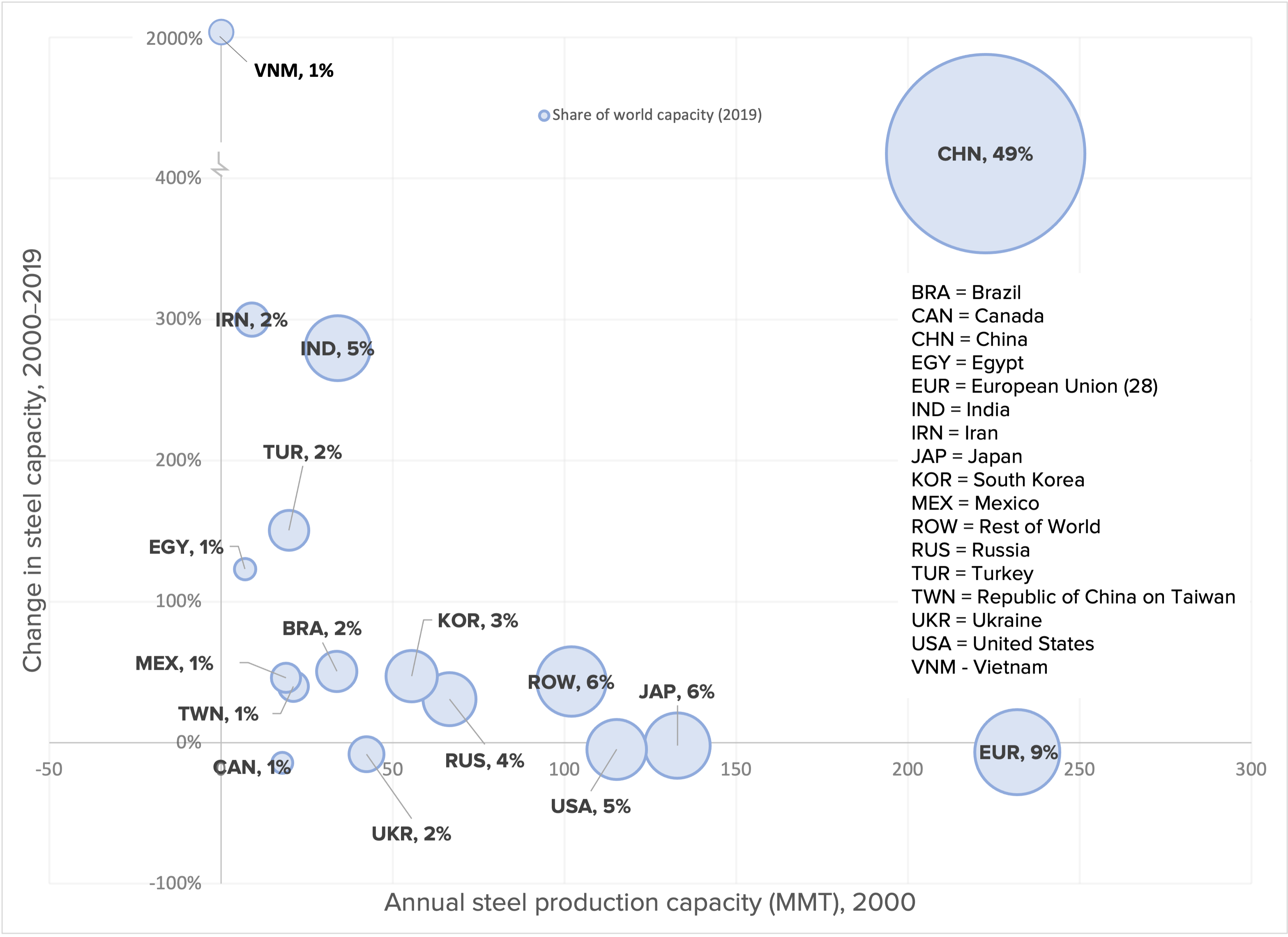
Note: The figure plots each country's steel production capacity in 2000 on the horizontal axis against the percentage growth in capacity from 2000 to 2019 on the vertical axis. The bubble sizes reflect each country’s relative share of global production capacity in 2019.
Source: OECD (2020a).
A multilateral solution to the chronic problem of global excess steel capacity remains essential. But until that time, the inefficacy of market mechanisms to address surplus overcapacity and national policy distortions introduced by foreign trade partners will continue plaguing U.S. steel producers, risking the industry’s survival at a scale necessary to meet national security demands.
Section 232 measures improve industry conditions, spur investments and jobs
Given that the problem of global excess capacity for U.S. steel producers is clear, policymakers should ask: “Are Section 232 measures on imported steel working to improve their conditions?” In considering this question, it is important to understand that the effectiveness of relief has been undermined by considerable “leakage” from Commerce-granted exclusions and broad countrywide exclusions that have curtailed tariff coverage on imported steel. Nevertheless, our analysis demonstrates that Sec. 232 measures remain critical to the long-term prospects of U.S. steel producers. A survey of publicly available sources reveals that following implementation of Sec. 232 measures, U.S. steel producers announced new investments, upgrades, plant expansions, and reopenings of idled facilities in at least 15 states, including plans to invest more than $15.7 billion in new or upgraded steel facilities, creating at least 3,200 direct new jobs, many of which are now poised to come online (see Appendix Table 1A). In addition, more than $5.9 billion was invested in plant acquisitions by nine firms, as part of industry restructuring to increase efficiency, preserving additional jobs at those facilities (see Appendix Table 1B).8
Individual anecdotes provide a suggestive initial glimpse at the effects of Sec. 232 steel import measures. But a more systematic assessment of available data demonstrates that the import measures coincided with improving conditions for U.S. producers—prior to the pandemic-related global recession beginning in 2020. Relief from the pressure of anti-competitive steel imports facilitated recovery of industrywide sales margins (a measure of profitability), production and capacity utilization rates, and a resurgence of new investment in steel industry fixed assets. Importantly, as discussed in the next section, these measures achieved improvements for U.S. steel producers without causing harm to downstream consumers of steel products in the United States.
From the trough of the Great Recession in 2009, U.S. steel imports rose sharply from 14.7 MMT to 40.2 MMT by 2014, as seen in Figure C. A series of nearly 69 new anti-dumping and countervailing duty determinations between 2014 and 2016 curbed the inflow of steel imports to 30 MMT in 2016—temporarily (USITC 2021).9 However, many foreign producers evaded these import surge measures by relocating steel production and processing to third countries, and imports climbed once again, reaching 34.5 MMT in 2017. But the Sec. 232 measures successfully slowed the pace of imports in 2018 and 2019, when imports fell to just 25.3 MMT. Overall, the volume of steel imports fell 27% between 2017 and 2019—before the pandemic’s “Great Lockdown” slowed U.S. and global economic activity. Separate data analysis shows that import penetration of the U.S. steel market fell to 26% of all steel consumed in the United States in 2019, from 35% in 2017. As a result, the rate of capacity utilization for U.S. steel producers rose to 80% in 2019 from 72% in 2017 (WSA 2020a; OECD 2020a). Commerce (BIS 2018) found that an 80% capacity utilization, sustained over the business cycle, is a critical threshold for U.S. steel producers to achieve long-term financial viability.
U.S. import penetration trend sets stage for Section 232 steel measures: U.S. imports of steel products by volume, 2009–2020
| Millions of metric tons (MMT) | |
|---|---|
| 2009 | 14.7 |
| 2010 | 21.7 |
| 2011 | 25.9 |
| 2012 | 30.4 |
| 2013 | 29.2 |
| 2014 | 40.2 |
| 2015 | 35.1 |
| 2016 | 30.0 |
| 2017 | 34.5 |
| 2018 | 30.6 |
| 2019 | 25.3 |
| 2020* | 18.8 |
* 2020 is a preliminary annual estimate.
Source: U.S. Census Bureau 2020b.
Sec. 232 measures placing tariffs and quotas on foreign steel products were intended to create some breathing room for U.S. steel producers to recover market share and sustainable financial conditions enabling them to increase domestic production—which they did. The Sec. 232 measures have afforded the U.S. steel industry an opportunity to recover to a level of financial performance not experienced since before the Great Recession (Figure D), although this recovery has been undermined as exemptions from Sec. 232 measures allowed “leakage” of uncovered imports, and as recession from the pandemic’s 2020 Great Lockdown set in. Following the Great Recession of 2007–2009, U.S. steel producers strained to achieve profitability. From the third quarter of 2009 through 2016, net income for the U.S. steel industry averaged just $73 million. Over the same period, net income as a share of sales—a measure of profitability—averaged 0%. In 2018, the year Sec. 232 measures were first imposed, net income in the steel industry reached $7.9 billion, or 6.4% of sales—its highest level since the real estate construction boom that preceded the Great Recession. Since then, however, the domestic industry has faced serious challenges. In 2019, the industry’s net income receded to $2.9 billion, and in 2020 it sunk back into negative territory, posting losses with the pandemic-induced global recession.
Steelmaker incomes recover with Section 232 import measures: U.S. steel producers' net income, annual and as a share of sales, 2001–2020
| Net income | Income/sales | |
|---|---|---|
| 2001 | -$7 | -8.6% |
| 2002 | -$2 | -2.9% |
| 2003 | -$3 | -4.1% |
| 2004 | $9 | 7.8% |
| 2005 | $9 | 7.6% |
| 2006 | $12 | 8.8% |
| 2007 | $9 | 6.4% |
| 2008 | $5 | 3.5% |
| 2009 | -$7 | -7.7% |
| 2010 | -$1 | -0.9% |
| 2011 | $3 | 2.5% |
| 2012 | $3 | 2.3% |
| 2013 | $0 | 0.3% |
| 2014 | $2 | 1.9% |
| 2015 | -$4 | -3.6% |
| 2016 | $1 | 1.0% |
| 2017 | $4 | 3.7% |
| 2018 | $8 | 6.4% |
| 2019 | $3 | 2.5% |
| 2020* | -$1 | -1.5% |
Note: 2020 data includes the first quarter through the third quarter.
Source: U.S. Census Bureau 2021; Bureau of Labor Statistics 2021b.
U.S. steel producers recovered with the Sec. 232 measures, bringing idled capacity back online with expectations for improving market conditions. However, more recently, the erosion of import coverage under Sec. 232 measures has coincided with declining prices and financial performance in the industry. Although the Sec. 232 measures initially covered all steel imports, Commerce has granted nearly 108,000 product exclusion requests from Sec. 232 measures as of July 2020 (CRS 2020; U.S. Department of Commerce 2021). A number of significant steel-producing countries, including Argentina, Brazil, Canada, Mexico, and South Korea, also obtained outright exemptions from Sec. 232 measures or quantitative quotas to replace import tariffs. These exclusions and exemptions significantly curtailed the coverage of Section 232 measures, although the measures remain significant in reversing the trend of declining viability of the U.S. steel industry. Today, a majority of steel products are imported to the United States either on a duty-free basis or under Sec. 232 product exclusions.
The U.S. steel industry’s initial recovery under Sec. 232 measures and the expectations of relief from conditions of chronic global excess capacity helped draw new investments into U.S. steel production (Figure E). New investment, adjusted for inflation, surpassed $5 billion in 2018 and reached nearly $5.9 billion in 2019. However, the dwindling coverage of Sec. 232 measures mentioned above and resulting decline in net income seen in Figure D will make it difficult for the industry to sustain this investment trend and could put many producers in further financial jeopardy. As discussed earlier, capital-intensive investments to upgrade and expand production are long-lived fixed costs that only can be reversed at prohibitively high cost. Firms that have made substantial new investments under the expectations of strong domestic demand and continuing Sec. 232 import relief may be deterred from future investments in technological upgrading and be squeezed by debt service commitments; those exploring expansion will likely shelve their plans.
U.S. capital investments in steel rise sharply following Sec. 232 measures: Real capital expenditures, 2001–2019
| Equipment | Structures | |
|---|---|---|
| 2001 | $1,696 | $507 |
| 2002 | $1,301 | $234 |
| 2003 | $1,657 | $454 |
| 2004 | $1,766 | $311 |
| 2005 | $1,881 | $592 |
| 2006 | $2,285 | $713 |
| 2007 | $2,859 | $686 |
| 2008 | $3,595 | $708 |
| 2009 | $4,700 | $782 |
| 2010 | $4,560 | $1,324 |
| 2011 | $4,502 | $1,646 |
| 2012 | $3,497 | $1,867 |
| 2013 | $5,857 | $1,347 |
| 2014 | $3,094 | $795 |
| 2015 | $3,236 | $664 |
| 2016 | $2,180 | $578 |
| 2017 | $2,106 | $987 |
| 2018 | $3,197 | $1,851 |
| 2019 | $3,822 | $2,028 |
Sources: U.S Census Bureau 2020a; Bureau of Economic Analysis 2021.
Despite a 25% tariff, the Sec. 232 measures had a limited effect on U.S. import prices of steel products, as seen in Figure F. The product categories in Figure F represent roughly three-fourths of total U.S. steel imports. Unit prices for imports of most steel products increased from 2017 to 2018—the year Sec. 232 import measures began. But then, import prices fell in 2019 and again in 2020, such that overall, averaged across all products, the import price of steel fell to $833 per metric ton in 2020 from $845 per metric ton in 2017.
Section 232 remedies have negligible effects on the real price of steel imports: Unit price of U.S. steel imports, inflation-adjusted, 2007 and 2016–2020
| Real $2020q3 | 2007 | 2016 | 2017 | 2018 | 2019 | 2020 |
|---|---|---|---|---|---|---|
| All steel products | $1,080 | $778 | $848 | $922 | $905 | $833 |
| Blooms, billets, and slabs | $671 | $455 | $518 | $597 | $566 | $507 |
| Sheets and strip, galvanized hot dipped | $948 | $804 | $886 | $926 | $928 | $902 |
| Oil country goods | $1,431 | $1,124 | $991 | $1,133 | $1,131 | $1,103 |
| Sheets, cold rolled | $1,545 | $897 | $921 | $982 | $946 | $925 |
| Sheets, hot rolled | $674 | $538 | $640 | $719 | $635 | $567 |
| Wire rods | $712 | $580 | $636 | $778 | $784 | $765 |
| Bars—reinforcing | $617 | $402 | $471 | $561 | $504 | $467 |
| Plates in coils | $944 | $588 | $720 | $754 | $700 | $625 |
| Bars—hot rolled | $1,090 | $931 | $955 | $1,025 | $1,076 | $1,036 |
| Sheets and strip, all other coated materials | $1,067 | $825 | $942 | $978 | $979 | $990 |
Sources: U.S. Census Bureau 2020b; Bureau of Labor Statistics 2021b.
Sec. 232 import measures coincided with and contributed to an increase in prices for steel products in the U.S. market, as can be seen in Figure G, comparing prices paid to domestic steel producers relative to those paid by U.S. steel consumers purchasing comparable products on international markets for import. Unsurprisingly, both U.S. producer and import prices follow a common trend, although imports generally are lower priced than U.S.-made steel, as excess capacity and trade-distorting foreign government policies depress global prices. As the world emerged from the Great Recession in July 2009, particularly with China’s outsized stimulus investments in infrastructure and real estate construction (Hersh 2014), steel prices around the world began rising sharply. Steel demand was so strong that it pushed up prices for key steel inputs globally, including iron ore and coal (World Bank 2020). Then, as discussed in Section 2 above, expanded world steel production and surplus capacity through the middle of the last decade began driving prices down.
Global markets, not Section 232 measures, drive steel prices: U.S. producer and imported steel prices, 2009–2020
| Date | Steel products, import prices | Steel products, producer prices |
|---|---|---|
| 2009-01-01 | 208.0 | 193.8 |
| 2009-02-01 | 201.1 | 185.9 |
| 2009-03-01 | 184.1 | 181.4 |
| 2009-04-01 | 178.1 | 170.2 |
| 2009-05-01 | 168.9 | 165.9 |
| 2009-06-01 | 165.0 | 166.2 |
| 2009-07-01 | 166.6 | 169.5 |
| 2009-08-01 | 169.4 | 175.5 |
| 2009-09-01 | 177.5 | 182.8 |
| 2009-10-01 | 180.5 | 188.3 |
| 2009-11-01 | 181.6 | 184.9 |
| 2009-12-01 | 179.0 | 185.1 |
| 2010-01-01 | 182.3 | 190.5 |
| 2010-02-01 | 185.8 | 196.3 |
| 2010-03-01 | 195.7 | 203.1 |
| 2010-04-01 | 205.1 | 211.7 |
| 2010-05-01 | 209.3 | 219.6 |
| 2010-06-01 | 213.1 | 222.0 |
| 2010-07-01 | 212.1 | 213.5 |
| 2010-08-01 | 208.5 | 206.9 |
| 2010-09-01 | 205.0 | 207.2 |
| 2010-10-01 | 203.3 | 207.8 |
| 2010-11-01 | 206.5 | 206.5 |
| 2010-12-01 | 203.2 | 208.3 |
| 2011-01-01 | 210.3 | 214.8 |
| 2011-02-01 | 218.7 | 227.4 |
| 2011-03-01 | 233.7 | 234.0 |
| 2011-04-01 | 239.4 | 240.1 |
| 2011-05-01 | 244.7 | 240.5 |
| 2011-06-01 | 243.9 | 237.9 |
| 2011-07-01 | 244.0 | 237.9 |
| 2011-08-01 | 241.5 | 237.6 |
| 2011-09-01 | 241.0 | 237.3 |
| 2011-10-01 | 234.9 | 236.2 |
| 2011-11-01 | 232.8 | 234.8 |
| 2011-12-01 | 230.2 | 233.7 |
| 2012-01-01 | 226.5 | 234.5 |
| 2012-02-01 | 227.1 | 236.2 |
| 2012-03-01 | 226.6 | 234.8 |
| 2012-04-01 | 226.2 | 234.3 |
| 2012-05-01 | 224.7 | 232.8 |
| 2012-06-01 | 220.9 | 227.5 |
| 2012-07-01 | 218.2 | 223.5 |
| 2012-08-01 | 212.3 | 217.5 |
| 2012-09-01 | 207.8 | 220.3 |
| 2012-10-01 | 203.0 | 215.7 |
| 2012-11-01 | 202.0 | 213.5 |
| 2012-12-01 | 198.6 | 215.0 |
| 2013-01-01 | 196.6 | 214.4 |
| 2013-02-01 | 198.9 | 212.8 |
| 2013-03-01 | 199.2 | 211.6 |
| 2013-04-01 | 198.4 | 212.1 |
| 2013-05-01 | 197.6 | 209.5 |
| 2013-06-01 | 198.0 | 209.1 |
| 2013-07-01 | 197.0 | 209.9 |
| 2013-08-01 | 197.8 | 209.8 |
| 2013-09-01 | 195.5 | 209.2 |
| 2013-10-01 | 197.9 | 210.8 |
| 2013-11-01 | 198.7 | 212.9 |
| 2013-12-01 | 201.1 | 213.8 |
| 2014-01-01 | 201.7 | 215.1 |
| 2014-02-01 | 204.8 | 215.8 |
| 2014-03-01 | 207.1 | 214.4 |
| 2014-04-01 | 205.7 | 216.0 |
| 2014-05-01 | 205.8 | 217.0 |
| 2014-06-01 | 205.3 | 217.9 |
| 2014-07-01 | 205.4 | 218.1 |
| 2014-08-01 | 204.5 | 218.9 |
| 2014-09-01 | 204.7 | 219.2 |
| 2014-10-01 | 204.5 | 218.5 |
| 2014-11-01 | 203.0 | 217.5 |
| 2014-12-01 | 201.0 | 215.3 |
| 2015-01-01 | 195.9 | 212.8 |
| 2015-02-01 | 189.5 | 207.0 |
| 2015-03-01 | 184.5 | 203.0 |
| 2015-04-01 | 173.5 | 196.7 |
| 2015-05-01 | 167.6 | 192.6 |
| 2015-06-01 | 164.9 | 191.8 |
| 2015-07-01 | 162.0 | 190.5 |
| 2015-08-01 | 162.1 | 188.9 |
| 2015-09-01 | 159.3 | 186.6 |
| 2015-10-01 | 154.5 | 182.9 |
| 2015-11-01 | 149.9 | 177.6 |
| 2015-12-01 | 146.4 | 173.5 |
| 2016-01-01 | 139.7 | 171.9 |
| 2016-02-01 | 138.8 | 170.6 |
| 2016-03-01 | 139.0 | 170.4 |
| 2016-04-01 | 143.9 | 174.5 |
| 2016-05-01 | 151.4 | 181.0 |
| 2016-06-01 | 159.8 | 185.0 |
| 2016-07-01 | 167.9 | 187.9 |
| 2016-08-01 | 170.8 | 191.1 |
| 2016-09-01 | 165.6 | 189.4 |
| 2016-10-01 | 163.6 | 186.7 |
| 2016-11-01 | 160.7 | 185.9 |
| 2016-12-01 | 162.0 | 188.5 |
| 2017-01-01 | 172.5 | 193.1 |
| 2017-02-01 | 180.6 | 198.5 |
| 2017-03-01 | 185.1 | 202.1 |
| 2017-04-01 | 186.8 | 203.6 |
| 2017-05-01 | 187.8 | 206.4 |
| 2017-06-01 | 186.1 | 206.9 |
| 2017-07-01 | 184.4 | 210.0 |
| 2017-08-01 | 185.6 | 204.1 |
| 2017-09-01 | 187.4 | 205.2 |
| 2017-10-01 | 193.2 | 203.5 |
| 2017-11-01 | 194.8 | 201.6 |
| 2017-12-01 | 191.7 | 202.6 |
| 2018-01-01 | 195.3 | 202.9 |
| 2018-02-01 | 200.4 | 207.5 |
| 2018-03-01 | 207.6 | 212.0 |
| 2018-04-01 | 214.8 | 217.3 |
| 2018-05-01 | 220.3 | 226.0 |
| 2018-06-01 | 218.9 | 231.9 |
| 2018-07-01 | 219.7 | 236.0 |
| 2018-08-01 | 219.6 | 241.0 |
| 2018-09-01 | 221.2 | 244.2 |
| 2018-10-01 | 219.8 | 242.2 |
| 2018-11-01 | 216.5 | 243.2 |
| 2018-12-01 | 216.4 | 241.7 |
| 2019-01-01 | 211.7 | 239.3 |
| 2019-02-01 | 208.3 | 233.4 |
| 2019-03-01 | 207.4 | 233.7 |
| 2019-04-01 | 212.8 | 229.9 |
| 2019-05-01 | 212.5 | 228.1 |
| 2019-06-01 | 209.6 | 223.6 |
| 2019-07-01 | 205.5 | 217.8 |
| 2019-08-01 | 205.3 | 214.7 |
| 2019-09-01 | 205.1 | 213.4 |
| 2019-10-01 | 198.6 | 211.1 |
| 2019-11-01 | 193.5 | 206.2 |
| 2019-12-01 | 187.9 | 203.1 |
| 2020-01-01 | 187.2 | 203.0 |
| 2020-02-01 | 190.1 | 203.1 |
| 2020-03-01 | 187.8 | 204.6 |
| 2020-04-01 | 187.1 | 203.1 |
| 2020-05-01 | 179.3 | 197.9 |
| 2020-06-01 | 177.8 | 196.7 |
| 2020-07-01 | 175.7 | 196.0 |
| 2020-08-01 | 178.2 | 192.5 |
| 2020-09-01 | 181.4 | 191.7 |
| 2020-10-01 | 185.1 | 194.3 |
| 2020-11-01 | 190.8 | 199.7 |
| 2020-12-01 | 193.0 | 207.2 |
Source: Bureau of Labor Statistics 2021a and 2021c.
Following implementation of Sec. 232 measures, Figure G shows domestic steel prices rose faster than U.S. import prices. This is due to a combination of the Sec. 232 measures, other trade remedies—including anti-dumping and countervailing duty orders—and the appreciation in value of the U.S. dollar relative to foreign currencies, making foreign products comparatively less expensive in dollar terms. These factors drove a wedge between domestic and foreign prices, which enabled U.S. steelmakers to achieve more sustainable operating margins. As input prices again eased in late 2018, steel prices fell in the U.S. market and globally—although they likely would have fallen further were it not for Sec. 232 import measures.
In recent months, U.S. and foreign steel prices are on the upswing—likely a temporary phenomenon caused by the lag between increasing demand as parts of the world economy recover from the Great Lockdown and the re-employment of steelmaking capacity—which, for blast furnace operations in particular, can take time and may occur only after market conditions create confidence that a facility can operate at a high level of capacity for a sustained period. In this environment, maintenance of Sec. 232 import measures will remain critical to ensuring the economic stability and financial viability of the U.S. industry. Country- and product-specific trade remedies, though significant, on their own have proven insufficient to abate the risk to the U.S. steel industry from anti-competitive imports and chronic excess production capacity.
Steel consumers face negligible effects from Section 232 measures
An important concern in assessing the impacts of Sec. 232 measures on imported steel products is how these measures affect downstream industries and consumers of products that use steel inputs. Indeed, as Sec. 232 measures were going into effect, a group of business lobbying associations representing downstream users sent a joint letter to the U.S. Trade Representative expressing this concern and claiming “significant harm” from this policy (Industry Week 2018). Our analysis in this section shows this claim proved incorrect.
Critics of import measures more broadly, including those levied in 2018 against China for unfair trade practices pertaining to technology transfer, intellectual property, and innovation (USTR 2018), often point to a recent Federal Reserve study purporting to find that tariffs are associated with negative outcomes for the U.S. manufacturing sector (Flaaen and Pierce 2019). However, this analysis should be treated with a healthy dose of skepticism due to myriad methodological issues that introduce statistical bias and call into question the validity of their findings.10 Weaknesses of Flaaen and Pierce’s (2019) results are illustrated in their own Figures 4 and B3, which demonstrate that import protection has no statistically significant impact on manufacturing employment, industrial output, or producer prices for virtually all of the period under consideration.
Given the inherent shortcomings of Flaaen and Pierce 2019, we implement an empirical strategy focused more narrowly on steel products and explicitly evaluating the causal effect of changes in the price of steel inputs on the prices of goods using steel. Our econometric analysis demonstrates that this relationship ranges from statistically insignificant (i.e., not statistically different from zero effect) to negligible. In other words, the statistical evidence does not support claims of harm from Sec. 232 measures that were predicted by certain steel-using businesses. This fact should not be surprising: Even in the downstream industries consuming the most steel, steel inputs amount to a minor share of overall production costs.
Harm to downstream industries would occur if Sec. 232 measures significantly increased steel prices, causing increased costs for producers or consumers of primary steel-containing goods, and then those costs squeezed profit margins or consumer welfare—by forcing consumers to either pay more for or consume less of a given product. To assess this linkage between steel input prices and end-user prices, we employ standard, related, and time-tested econometric techniques known as Granger causality analysis and vector autoregression (Granger 1969; Sims 1980). Vector autoregression (VAR) is a statistical method for modeling a system of variables and their interrelationship and co-evolution over time. In this case, we model (1) the price of primary steel inputs, (2) the price of steel-consuming products, and (3) the effective federal funds rate.11
Granger causality analysis uses the VAR model to test for evidence of a statistically causal relationship between the variables in the model. If past values of variable 1 are shown to significantly predict current values of variable 2, then it can be concluded that variable 1 “Granger-causes” variable 2. While the price variable used in this modeling includes the effects of Sec. 232 tariffs and quotas, the results of the statistical test are not limited to the effects of Sec. 232 measures, but rather evaluate whether a change in prices resulting from any factor causes a change in the price of the steel-using good. Technical discussion of this methodology and detailed results are presented in Appendix 2.
We summarize the results of this causal analysis in Table 1. Each row of the table presents a separate VAR model relating the price of a steel-containing product with the price of its most relevant primary steel input(s) and reports the causal effect found on end-use product prices. The end-use products investigated represent the U.S. industries consuming the largest volume of steel products: nonresidential construction, motor vehicles, motor vehicle parts, construction machinery, electrical equipment and household appliances, and food processing (food consumed at home). We also evaluate the possible impacts of Sec. 232 steel measures at a broader level by modeling the effects of steel product prices on aggregated prices for durable goods.
As shown in Table 1, this analysis finds no discernible effect of steel prices causing price changes in new motor vehicles, motor vehicle parts, construction machinery, electrical equipment and household appliances, or, broadly, durable goods. These results, therefore, suggest that even if Sec. 232 measures caused an increase in the price of steel products, one would not expect a significant impact on the price of downstream goods. For prices of nonresidential construction goods and food consumed at home, the price of relevant steel inputs is found to be statistically significant in causing changes in the prices of steel-using products.12 While finding a statistical relationship between steel input prices and final goods prices, the same analysis shows that the economic significance of the impact is negligible: A 1% increase in steel input prices caused a 0.1% change in the price of construction goods and a less than 0.05% change in the price of food at home. However, as discussed in Appendix 2, causal analysis suggests the relationship between steel inputs and construction goods actually runs in the opposite direction, with demand for construction goods driving prices in the market for intermediate inputs.
Effects of Section 232 steel measures on end-use products
| End-use product | Primary steel inputs | Total steel inputs as share of gross production costs | Causal effect on end-use goods prices |
|---|---|---|---|
| Durable goods (personal consumption expenditures) | Cold-rolled steel sheet and strip; hot-rolled steel sheet and strip, including tin mill products; hot-rolled steel bars, plates, and structural shapes, carbon | — | No statistical effect |
| New motor vehicles (consumer) | Cold-rolled steel sheet and strip | 4.3% | No statistical effect |
| Motor vehicle parts (producer) | Hot-rolled steel sheet and strip, including tin mill products; Hot-rolled steel bars, plates, and structural shapes, carbon | 9.8% | No statistical effect |
| Nonresidential construction goods | Hot-rolled steel bars, plates, and structural shapes, carbon | 1.9% | Statistically significant but economically insignificant effect (a 1% change in steel causes a 0.1% change) |
| Construction machinery | Hot-rolled steel bars, plates, and structural shapes, carbon | 8.2% | No statistical effect |
| Electrical equipment and household appliances | Cold-rolled steel sheet and strip; Steel wire, carbon | 4.7% | No statistical effect |
| Food at home | Hot-rolled steel sheet and strip, including tin mill products | 1.0% | Statistically significant but economically insignificant effect (a 1% change in steel causes <0.05% change) |
Source: Authors' analysis of BLS (2020, 2021b, 2021c, and 2021d) and FRED (2021) data.
To recap, while conceptually a relationship exists between input prices and final goods prices, econometric analysis of the causal relationship between prices finds effects ranging from statistically zero to essentially nothing. Sec. 232 measures simply did not have a meaningful, real-world impact on prices for steel-consuming products. This fact should not be surprising. Even in the industries that consume the largest volumes of steel products, steel is just one cost in a long list of inputs to production. Despite these industries accounting for the lion’s share of steel consumption in the U.S. economy, the cost of their steel inputs is minor relative to their gross production. As shown in Table 1, the steel content as a share of total production ranges from 1% in food consumed at home to 9.8% in the motor vehicle parts industries. Illustrating the point in dollar terms, the average passenger car contains roughly 900 kg of steel (WSA n.d.). At a current cost of $1,048 per metric ton, the steel inputs amount to just 2% of the sales price for the average new U.S. car (Steel Benchmarker 2020; Kelley Blue Book 2020). In contrast, electronics components make up roughly 40% of a new car’s price (Deloitte 2019).
Retreating from Section 232 measures would squeeze vulnerable producers, increase greenhouse gas emissions
Thus far, we have seen that Sec. 232 import measures have helped improve market conditions for U.S. steel producers amid chronic global excess capacity that threatens their financial viability. We also have seen that the impact of these measures on steel-consuming U.S. industries has ranged from zero to economically insignificant. Furthermore, the benefits of this policy have eroded since it began as more steel imports have been exempted from the Sec. 232 regime. As the world looks to move forward from the economic shock of the Great Lockdown caused by COVID-19, it is clear that eliminating or even further relaxing the steel import measures likely would pose serious economic consequences for U.S. steel producers. Two important points are noteworthy here.
First, a slow and uneven recovery from the 2020 economic downturn is expected, with global demand for steel products uncertain. The International Monetary Fund (IMF) recently revised down its global economic growth forecast for 2021; it projects “limited progress toward catching up to the [expected] path of economic activity for 2020–2025” (IMF 2020).13 Families around the world have suffered deep economic scarring from lost jobs and income and depleted savings—not to mention, tragically, the many who have lost prime wage-earners. Millions of people worldwide who contracted the virus are likely to suffer long-term effects, reducing prospects for employment and earnings and allocating a larger share of disposable income toward health care services and away from goods consumption. At the same time, the downturn and its long-lasting effects have dampened public-sector revenues at a time when governments have undertaken unprecedented expenditures meeting the public health crisis and providing social protections. The enduring effects of this shock will dampen, in the near term, a recovery of household consumption and, in turn, business investment. In the longer term, the human toll will dampen prospects for economic potential, dragging down investments in human and fixed asset capital and the productivity growth these investments provide.
Economic recovery, of course, is contingent on how well world governments abate the global health crisis, but it is clear that even under optimistic scenarios, demand for steel production will remain muted for some time. U.S. steel demand declined 16% in 2020, and in 2021 it is expected to remain more than 10% below 2019 levels (WSA 2020c). Globally, steel demand declined 6.4% from 2019 to 2020 and is forecast to remain nearly 3% below 2019 levels (OECD 2020c). At the same time, countries have not retreated from policy efforts to prop up national steel industries (see text box, “Widespread government interventions drive unfair trade in steel products”) and are continuing to install additional productive capacity. The OECD (2020b) projects that by 2022, producers will add as much as another 3% of steelmaking capacity worldwide, concentrated in Asia and the Middle East.
Together, these trends point to increased excess steelmaking capacity and lower capacity utilization rates that would drive prices down and squeeze U.S. steel producers who face competition with imports produced on a noncommercial basis. These are exactly the pressures Sec. 232 measures are designed to address, in the absence of multilateral agreements to manage excess capacity. Retreating from these measures now, particularly after many U.S. companies committed to new investments in production (Figure E; Appendix 1), would leave U.S. steel producers in untenable financial positions, further jeopardizing their capacity to meet national security needs.
Second, a significant ancillary benefit of Sec. 232 import measures has been to divert steel production to more environmentally sustainable producers. Relaxing Sec. 232 measures would reverse this progress as the world looks to decarbonizing and achieving net-neutral emissions by midcentury. The U.S. steel industry is one of the cleanest and most energy-efficient steel industries globally. A 2019 report measuring the CO2 emissions intensity of steel industries in 15 major steel-producing countries ranked U.S. steelmakers among the least CO2 intensive industries—with industries in Brazil, Canada, China, France, Germany, India, Japan, South Korea, and other countries having higher CO2 emissions intensity (Hasanbeigi and Springer 2019, Figure 14).
Even this analysis understates that difference in environmental impact, as it does not account for the substantial pollution from ocean freight required to transport raw materials and finished products in supply-chain webs around the world before foreign steel products can reach the U.S. market (ENVI 2020). If Sec. 232 measures are relaxed, it is precisely the most polluting national steel industries, in countries that have rapidly expanded capacity at the expense of more efficient producers, that stand to capture marginal changes in market share. And as excess capacity further squeezes prices and profit margins, firms will face difficulty investing in new technologies to allow for greener steel production and will risk being shut out of markets as consumers develop preferences for low-carbon products.
Conclusion: The Section 232 trade measures helped slow the flood of unfair imports that was squeezing the U.S. steel industry without hurting downstream steel-using producers and consumers
Surging steel imports have undermined domestic steel production, prices, employment, profits, investments, and the fundamental health of the U.S. domestic steel industry. Global steel surpluses are the result of chronic global excess steelmaking capacity in major exporting countries. The steel Section 232 trade restraints imposed in 2018, including both tariffs and quotas on imports from selected countries, helped slow the flood of steel imports. Following imposition of these measures, U.S. steel output, employment, capital investment, and financial investment all improved.
Meanwhile, statistical analysis in this report has demonstrated that Section 232 measures have had no economically significant impacts on the prices of downstream products. Despite the benefits of the Section 232 tariffs for the domestic steel industry and its workers, and the minimal impacts of trade restraints on downstream industries, these measures have been progressively weakened by nearly 108,000 product-specific exclusions and broad tariff exemptions for a number of countries.
The domestic steel industry is just beginning to emerge from the depths of the COVID-19 recession with a steep hill to climb, given widening excess global steel capacity. With the right policies and major investments planned by the new administration in economic rebuilding, clean energy, and infrastructure construction, U.S. steel producers can be poised for a substantial upswing in employment, output, and investment that fuels growth in clean, efficient, state-of-the-art domestic steel production. The window to this opportunity could be slammed shut by the premature and unplanned elimination of the Section 232 import measures.
Acknowledgments
The authors thank Jori Kandra for technical and research assistance and Colleen O’Neill and Lora Engdahl for editing assistance. This research was made possible by support from the Partners for American-made Steel.
About the authors
Adam S. Hersh, Ph.D., is director of Washington Global Advisors, LLC, and a research associate at the Political Economy Research Institute, University of Massachusetts Amherst. Hersh was formerly chief economist for the Congressional Joint Economic Committee, Democratic staff; senior economist at the Franklin and Eleanor Roosevelt Institute and the Center for American Progress; a visiting scholar at Columbia University’s Initiative for Policy Dialogue and the Shanghai University of Finance and Economics; and a research fellow at the University College, London’s Institute for Innovation and Public Purpose. He is a contributing author with Joseph Stiglitz of Rewriting the Rules of the American Economy: An Agenda for Growth and Shared Prosperity (2015).
Robert E. Scott joined the Economic Policy Institute in 1996 and is currently director of trade and manufacturing policy research. His areas of research include international economics, trade, and manufacturing policies and their impacts on working people in the United States and other countries, the economic impacts of foreign investment, and the macroeconomic effects of trade and capital flows. He has published widely in academic journals and the popular press, including The Journal of Policy Analysis and Management, The International Review of Applied Economics, and The Stanford Law and Policy Review, as well as The Los Angeles Times, Newsday, USA Today, The Baltimore Sun, The Washington Times, and other newspapers. He has also provided economic commentary for a range of electronic media, including NPR, CNN, Bloomberg, and the BBC. Mr. Scott has a Ph.D. in economics from the University of California, Berkeley.
Endnotes
1. 19 U.S.C. §1862; https://www.law.cornell.edu/uscode/text/19/1862.
2. Adjusting Imports of Aluminum Into the United States, 83 Fed. Reg. 25849–25855 (March 15, 2018).
3. Adjusting Imports of Steel Into the United States, 83 Fed. Reg. 25857–25877 (March 15, 2018).
4. The capital-to-labor ratio for primary metals producers is 76% higher than for durable goods manufacturing industries overall. See BLS (2020).
5. This section is based, in part, on information summarized in Examples of Policies and Practices Contributing to the Global Excess Capacity Crisis, a report by the American Iron and Steel Institute and the Steel Manufacturers Association included at the end of this report.
6. There are two anti-dumping orders in place against Canadian steel products, and there are both anti-dumping and countervailing duty orders in place against wind towers, a major steel-using product. South Korean steel orders include six countervailing duty orders and 26 antidumping orders. EPI analysis of USITC (2021).
7. Countries receiving Chinese direct foreign investment in steel include Cambodia, Malaysia, Indonesia, Myanmar, Pakistan, the Philippines, Bolivia, Vietnam, the United Kingdom, and the Netherlands. See OECD (2020b).
8. These are direct steelmaking jobs; the investments would also generate indirect employment through the goods and services procured in expansion products, as well as induced employment generated by the incomes from direct and indirect employees.
9. The USITC (2021) lists 276 anti-dumping and countervailing duties in effect on steel products (categories ISM, ISO, and ISP) as of December 28, 2020, and of those, 69 orders went into effect between 2014 and 2016.
10. It is worth briefly considering several reasons why. First, the core explanatory variable—“import protection”—ignores the actual incidence and evolution of protection over time as more products received exclusions from tariffs. Second, their statistical model explicitly embraces violations of the core assumptions on which the statistical method is built, biasing the results. In particular, equation 7 specifies measures of import protection, input costs, and foreign retaliation as “independent” variables associated with the dependent variables of manufacturing employment, output, and producer prices. In fact, as Flaaen and Pierce appropriately theorize, input costs and foreign retaliation are, at least in part, caused by import protection. Finally, Flaaen and Pierce’s analysis conflates the effects of Sec. 232 import measures with Sec. 301 trade remedies. Conditions of chronic excess global steel capacity—explained in Section 2 above—mean that market conditions are significantly different for steel products than for other manufactured goods, suggesting that pooling data for steel products and other manufactured goods more broadly is inappropriate and may bias estimates of the statistical significance.
11. The federal funds rate—the interest rate at which depository institutions borrow and lend federal balances held at Federal Reserve Banks—is the primary target for Federal Reserve monetary policy actions and is linked both in theory and in practice to changes in price levels as well as to the level of demand for goods and services across the economy.
12. The causal effect of steel prices on food-at-home prices shows only weak statistical significance, at the 90% probability threshold; the model for other significant goods found 95% to 99% probability.
13. What’s more, as dour as the IMF’s assessment is, their forecasts are notorious for being overly optimistic. See Rosnick and Weisbrot (2007).
14. Producer Price Index by Commodity: Metals and Metal Products: Iron and Steel (WPU101); Producer Price Index by Commodity: Metals and Metal Products: Cold Rolled Steel Sheet and Strip (WPU101707); Producer Price Index by Commodity: Metals and Metal Products: Hot Rolled Steel Sheet and Strip, Including Tin Mill Products (WPU101703); Producer Price Index by Commodity: Metals and Metal Products: Hot Rolled Steel Bars, Plates, and Structural Shapes (WPU101704); Producer Price Index by Commodity: Metals and Metal Products: Steel Wire (WPU101705); Consumer Price Index for All Urban Consumers: New Vehicles in U.S. City Average (CUUR0000SETA01); Producer Price Index by Commodity: Transportation Equipment: Motor Vehicles Parts (WPU1412); Producer Price Index by Industry: Construction Machinery Manufacturing (PCU333120333120); Producer Price Index by Commodity: Inputs to Industries: Net Inputs to Nonresidential Construction, Goods (WPUIP2312001); Producer Price Index by Industry: Electrical Equipment and Appliance Manufacturing (PCU335335); Consumer Price Index for All Urban Consumers: Food at Home in U.S. City Average (CUSR0000SAF11); Personal consumption expenditures: Durable goods (chain-type price index) (DDURRG3M086SBEA); and Effective Federal Funds Rate (FEDFUNDS).
15. Motor vehicle parts manufacturing requires significant inputs from both hot-rolled sheet and strip as well as hot-rolled bars, plates, and structural shapes. Electrical equipment and household appliances require significant inputs from both cold-rolled sheet and strip and carbon steel wire. Therefore, these products are modeled as a four-equation VAR of the form
![\left[\begin{array}{l} \triangle p_{t}^{1} \\ \triangle p_{t}^{2} \\ \triangle p_{t}^{3} \\ \triangle i_{t} \end{array}\right]=a_{0}+A_{1}\left[\begin{array}{c} \triangle p_{t-1}^{1} \\ \triangle p_{t-1}^{2} \\ \triangle p_{t-1}^{3} \\ \triangle i_{t-1} \end{array}\right]+\cdots+A_{k}\left[\begin{array}{c} \triangle p_{t-k}^{1} \\ \triangle p_{t-k}^{2} \\ \triangle p_{t-k}^{3} \\ \triangle i_{t-k} \end{array}\right]+\left[\begin{array}{c} \varepsilon_{1, t} \\ \varepsilon_{2, t} \\ \varepsilon_{3, t} \\ \varepsilon_{4, t} \end{array}\right]](https://s0.wp.com/latex.php?latex=%5Cleft%5B%5Cbegin%7Barray%7D%7Bl%7D++%5Ctriangle+p_%7Bt%7D%5E%7B1%7D+%5C%5C++%5Ctriangle+p_%7Bt%7D%5E%7B2%7D+%5C%5C++%5Ctriangle+p_%7Bt%7D%5E%7B3%7D+%5C%5C++%5Ctriangle+i_%7Bt%7D++%5Cend%7Barray%7D%5Cright%5D%3Da_%7B0%7D%2BA_%7B1%7D%5Cleft%5B%5Cbegin%7Barray%7D%7Bc%7D++%5Ctriangle+p_%7Bt-1%7D%5E%7B1%7D+%5C%5C++%5Ctriangle+p_%7Bt-1%7D%5E%7B2%7D+%5C%5C++%5Ctriangle+p_%7Bt-1%7D%5E%7B3%7D+%5C%5C++%5Ctriangle+i_%7Bt-1%7D++%5Cend%7Barray%7D%5Cright%5D%2B%5Ccdots%2BA_%7Bk%7D%5Cleft%5B%5Cbegin%7Barray%7D%7Bc%7D++%5Ctriangle+p_%7Bt-k%7D%5E%7B1%7D+%5C%5C++%5Ctriangle+p_%7Bt-k%7D%5E%7B2%7D+%5C%5C++%5Ctriangle+p_%7Bt-k%7D%5E%7B3%7D+%5C%5C++%5Ctriangle+i_%7Bt-k%7D++%5Cend%7Barray%7D%5Cright%5D%2B%5Cleft%5B%5Cbegin%7Barray%7D%7Bc%7D++%5Cvarepsilon_%7B1%2C+t%7D+%5C%5C++%5Cvarepsilon_%7B2%2C+t%7D+%5C%5C++%5Cvarepsilon_%7B3%2C+t%7D+%5C%5C++%5Cvarepsilon_%7B4%2C+t%7D++%5Cend%7Barray%7D%5Cright%5D&bg=ffffff&fg=000000&s=0 "\left[\begin{array}{l} \triangle p_{t}^{1} \\ \triangle p_{t}^{2} \\ \triangle p_{t}^{3} \\ \triangle i_{t} \end{array}\right]=a_{0}+A_{1}\left[\begin{array}{c} \triangle p_{t-1}^{1} \\ \triangle p_{t-1}^{2} \\ \triangle p_{t-1}^{3} \\ \triangle i_{t-1} \end{array}\right]+\cdots+A_{k}\left[\begin{array}{c} \triangle p_{t-k}^{1} \\ \triangle p_{t-k}^{2} \\ \triangle p_{t-k}^{3} \\ \triangle i_{t-k} \end{array}\right]+\left[\begin{array}{c} \varepsilon_{1, t} \\ \varepsilon_{2, t} \\ \varepsilon_{3, t} \\ \varepsilon_{4, t} \end{array}\right]")
where 

Appendix 1: New and expanded U.S. steel production under Section 232 measures capacity
Significant new, expanded, and restarted U.S. steel production since Section 232 measures
| Company | Facility | Additional capacity (metric tons) | Investment ($ millions) | Jobs created | |
|---|---|---|---|---|---|
| 1 | AM/NS Calvert | Calvert, AL, new EAF | 1,650,000 | $775 | TBD |
| 2 | Big River Steel | Brownsville, TX, new EAF | TBD | $1,600 | TBD |
| 3 | Big River Steel | Osceola, AR, doubled EAF and finishing capacity | 1,600,000 | $1,200 | TBD |
| 4 | Carpenter Technology | Reading, PA, new strip hot-rolling mill | NA | $100 | TBD |
| 5 | Charter Steel | Cuyahoga Heights, OH, new SBQ rolling mill | NA | $150 | 25 |
| 6 | Cleveland-Cliffs Inc. | Silver Bay, MN, new low-silica DR-grade pellets production | NA | $100 | NA |
| 7 | Cleveland-Cliffs Inc. | Toledo, OH, new HBI plant | NA | $940 | 160 |
| 8 | Commercial Metals Company | Durant, OK, new micro mill | 350,000 | $250 | 300 |
| 9 | Commercial Metals Company | Mesa, AZ, micro mill expansion | 500,000 | $300 | 185 |
| 10 | JSW USA
|
1,500,000 | $500 | TBD | |
| 11 | North Star BlueScope | Delta, OH, new EAF | 850,000* | $700 | NA |
| 12 | Nucor | Blytheville, AR, new 3rd gen. galvanizing line | NA | $275 | TBD |
| 13 | Nucor | Blytheville, AR, new specialty cold mill complex | NA | $245 | 100 |
| 14 | Nucor | Brandenburg, KY, new plate mill | 1,200,000 | $1,700 | 400 |
| 15 | Nucor | Convent, LA, DRI upgrade | NA | $200 | NA |
| 16 | Nucor | Frostproof, FL, new rebar micro mill | 350,000 | $240 | 250 |
| 17 | Nucor | Ghent, KY, flat-rolled mill expansion | 1,400,000 | $650 | 70 |
| 18 | Nucor | Ghent, KY, new hot band galvanizing line | NA | $200 | 75 |
| 19 | Nucor | Sedalia, MO, new rebar micro mill | 350,000 | $245 | 255 |
| 20 | Nucor | Bourbonnais, IL, full-range merchant bar quality mill | NA | $185 | 100 |
| 21 | PRO-TEC Coating Company (JV of U.S. Steel and Kobe) | Leipsic, OH, new CGL line | NA | $400 | TBD |
| 22 | SSAB | Mobile, AL, EAF upgrade | NA | $100 | 50 |
| 23 | Steel Dynamics Inc. | Sinton, TX, new EAF and finishing facilities | 3,000,000 | $1,900 | 625 |
| 24 | Steel Dynamics Inc. | Columbus, MS, new galvanizing line | NA | $142 | 45 |
| 25 | U.S. Steel | Fairfield, AL, new EAF | 1,600,000 | $215 | 150 |
| 26 | U.S. Steel | Granite City, IL, restart steelmaking | 1,500,000 | Not Stated | 500 |
| 27 | U.S. Steel | Gary, IN, upgrade steelmaking facilities | NA | $750 | NA |
| 28 | U.S. Steel | Mon Valley, PA, upgrade coke plant controls | NA | $200 | NA |
| 29 | U.S. Steel | Mon Valley, PA, new endless casting and rolling line, and cogen facility | NA | $1,500 | NA |
| 13 states | $15,762 | 3,290 |
*Additional is equivalent to 936,965 short tons; current is 2,100,000 short tons.
Notes: Additional capacity includes newly announced capacity or restarted basic oxygen furnace (BOF) or electric arc furnace (EAF) capacity, where available; does not include rolling mill, galvanizing or finishing capacity. Investment includes entries including significant new and expanded investments of $100+ million. Jobs created includes direct steel employment by company where available—does not include indirect jobs such as construction or contractors. SBQ refers to special bar quality. AM/NS Calvert is a joint venture of Arcelor Mittal and Nippon Steel Corp.; JSW steel is an OH steel co.; SSAB is a Swedish/US steel co.; ATI Metals is a specialty steel producer.
Sources: American Iron and Steel Institute; Steel Manufacturers Association. Compiled from public sources.
2018–2020 steel industry acquisitions
| Company | Description | Investment ($ millions) | |
|---|---|---|---|
| 1 | Cleveland-Cliffs Inc. | Multiple locations, acquire AK Steel | $1,100 |
| 2 | Cleveland-Cliffs Inc. | Multiple locations, acquire ArcelorMittal USA | $1,400 |
| 3 | Commercial Metals Company | Multiple locations, acquire USA assets of Gerdau | $600 |
| 4 | Liberty House Group | Multiple locations (GA, IL, NM, OH, SC, TX), acquire Keystone Consolidated Industries | $320 |
| 5 | Steel Dynamics, Inc. | Ashland, KY, acquire and reopen KY Electric Steel rolling mill | NA |
| 6 | Steel Dynamics, Inc. | Terra Haute, IN, acquire Heartland Steel Processing LLC | NA |
| 7 | Tenaris | Multiple locations, acquire IPSCO Tubulars | $1,067 |
| 8 | ATI | Vandergrift, PA, consolidate operations | $65-85 |
| 9 | U.S. Steel | Osceola, AR, acquire Big River Steel | $1,474 |
| $5,961 |
Sources: American Iron and Steel Institute; Steel Manufacturers Association. Compiled from public sources.
Appendix 2: Methodology for analyzing causal relationship between steel prices and steel-consuming industries
This appendix outlines the methodological approach for assessing how Sec. 232 measures on imported steel products may affect downstream industries and consumers of products that use steel inputs. Harm to downstream industries and consumers could occur if Sec. 232 measures caused an increase in prices for steel products paid by U.S. users of steel and if those price increases were passed through to producer or consumer prices for steel-embodying goods. In order to assess this possibility, we evaluate a more basic question: Do changes in prices of basic steel products cause changes in steel-using products? This question asks whether any change in steel prices is a significant determinant of goods prices that use steel as an intermediate input, irrespective of what factors cause a change in steel prices.
Data and methodology
To evaluate this question, we estimate reduced-form vector autoregressions (VARs) that model the variables of interest as an interrelated system that co-evolves over time (Sims 1980). The VAR is an attractive analytical tool because it does not force an assumed structural form onto the data. Each variable in the system is modeled jointly as a function of its past values and the past values of the other related variables in the system. After estimating the system, we can evaluate causal relationships between the variables by testing whether past values of one variable are statistically significant determinants of the current value of another variable, following Granger (1969).
Our variables of interest are (1) prices for steel products, (2) prices for steel-using products, and (3) the effective federal funds rate—the interest rate at which depository institutions borrow and lend reserve balances held at Federal Reserve Banks.14 This interest rate is the primary target for Federal Reserve monetary policy actions and is linked both in theory and in practice to changes in general price levels, as well as to the level of demand for goods and services across the economy via the Taylor Rule (Taylor 1993). Data are observed monthly and drawn from the Federal Reserve Bank of St. Louis’s FRED Economic Data, spanning December 2001 to January 2020, or two business cycle expansions, other than for steel wire, for which available data begin in July 2004. Univariate analysis with a modified Dickey-Fuller test (Cheung and Lai 1995) fails to reject the null hypothesis of a unit root for each variable under consideration. While the individual variables are nonstationary (integrated of order one, or first-difference stationary), tests with Johansen’s procedure show that there is no cointegration—or a stable, long-run relationship—between the variables (Johansen 1995), and the system can be modeled with a VAR, as opposed to a vector error correction model.
The VAR model consists of
![\left[\begin{array}{l} \Delta p_{t}^{1} \\ \Delta p_{t}^{2} \\ \Delta i_{t} \end{array}\right]=\alpha_{0}+A_{1}\left[\begin{array}{l} \Delta p_{t-1}^{1} \\ \Delta p_{t-1}^{2} \\ \Delta i_{t-1} \end{array}\right]+\cdots+A_{k}\left[\begin{array}{c} \Delta p_{t-k}^{1} \\ \Delta p_{t-k}^{2} \\ \Delta i_{t-k} \end{array}\right]+\left[\begin{array}{c} \varepsilon_{1, t} \\ \varepsilon_{2, t} \\ \varepsilon_{3, t} \end{array}\right]](https://s0.wp.com/latex.php?latex=%5Cleft%5B%5Cbegin%7Barray%7D%7Bl%7D++%5CDelta+p_%7Bt%7D%5E%7B1%7D+%5C%5C++%5CDelta+p_%7Bt%7D%5E%7B2%7D+%5C%5C++%5CDelta+i_%7Bt%7D++%5Cend%7Barray%7D%5Cright%5D%3D%5Calpha_%7B0%7D%2BA_%7B1%7D%5Cleft%5B%5Cbegin%7Barray%7D%7Bl%7D++%5CDelta+p_%7Bt-1%7D%5E%7B1%7D+%5C%5C++%5CDelta+p_%7Bt-1%7D%5E%7B2%7D+%5C%5C++%5CDelta+i_%7Bt-1%7D++%5Cend%7Barray%7D%5Cright%5D%2B%5Ccdots%2BA_%7Bk%7D%5Cleft%5B%5Cbegin%7Barray%7D%7Bc%7D++%5CDelta+p_%7Bt-k%7D%5E%7B1%7D+%5C%5C++%5CDelta+p_%7Bt-k%7D%5E%7B2%7D+%5C%5C++%5CDelta+i_%7Bt-k%7D++%5Cend%7Barray%7D%5Cright%5D%2B%5Cleft%5B%5Cbegin%7Barray%7D%7Bc%7D++%5Cvarepsilon_%7B1%2C+t%7D+%5C%5C++%5Cvarepsilon_%7B2%2C+t%7D+%5C%5C++%5Cvarepsilon_%7B3%2C+t%7D++%5Cend%7Barray%7D%5Cright%5D&bg=ffffff&fg=000000&s=0 "\left[\begin{array}{l} \Delta p_{t}^{1} \\ \Delta p_{t}^{2} \\ \Delta i_{t} \end{array}\right]=\alpha_{0}+A_{1}\left[\begin{array}{l} \Delta p_{t-1}^{1} \\ \Delta p_{t-1}^{2} \\ \Delta i_{t-1} \end{array}\right]+\cdots+A_{k}\left[\begin{array}{c} \Delta p_{t-k}^{1} \\ \Delta p_{t-k}^{2} \\ \Delta i_{t-k} \end{array}\right]+\left[\begin{array}{c} \varepsilon_{1, t} \\ \varepsilon_{2, t} \\ \varepsilon_{3, t} \end{array}\right]")
where 


The specific number 
The specific parameters estimated that define the structures of VARs are typically of less concern than how the system behaves when there is an exogenous change in one of the variables. In this case, we are concerned whether a change in the price 


Results
Appendix Table 2 reports the Wald test statistic χ2 and the associated probability for rejecting the null hypothesis of zero causal effect for each pair of prices. For the majority of end-use products considered, we find no statistical evidence that steel input prices affect the price of end-use products (<95% probability). This means that a change in steel prices is expected to have no effect on the price of end-use goods. We do find statistically significant causal effects (>95% probability) of steel input prices on the prices of nonresidential construction goods and food at home.
Granger causality test results: Effects of steel prices on end-use goods prices
| End-use product | Steel product(s) | k-lags | χ^2 | Probability of significance | Causality | Average effect of 1% price increase |
|---|---|---|---|---|---|---|
| Durable goods | Iron and steel | 1 | 3.5322 | 94.0% | Weak | 0.02% |
| Durable goods | Cold-rolled sheet and strip | 1 | 1.0615 | 69.7% | N | 0.00% |
| Hot-rolled sheet and strip, incl. tin mill products | 1 | 0.6951 | 59.6% | N | 0.00% | |
| Hot-rolled bars, plates, and structural shapes, carbon | 1 | 1.0796 | 70.1% | N | 0.00% | |
| New motor vehicles | Cold-rolled sheet and strip | 2 | 1.5724 | 54.4% | N | 0.00% |
| Motor vehicle parts | Hot-rolled sheet and strip, incl. tin mill products | 4 | 2.6699 | 38.6% | N | 0.00% |
| Hot-rolled bars, plates, and structural shapes, carbon | 4 | 5.8361 | 78.8% | N | 0.00% | |
| Construction machinery | Hot-rolled bars, plates, and structural shapes, carbon | 1 | 0.2072 | 35.1% | N | 0.00% |
| Nonresidential construction goods | Hot-rolled bars, plates, and structural shapes, carbon | 1 | 5.2682 | 97.8% | Y | 0.10% |
| Electrical equipment and household appliances | Cold-rolled sheet and strip | 2 | 1.6912 | 80.7% | N | 0.00% |
| Steel wire, carbon | 2 | 0.4380 | 49.2% | N | 0.00% | |
| Food at home | Hot-rolled sheet and strip, incl. tin mill products | 3 | 8.8442 | 96.9% | Y | 0.05% |
Source: Authors analysis of BLS (2021b, 2021c, and 2021d) and FRED (2021) data.
For end-use goods experiencing a causal effect of steel prices, we estimate the impact of a 1% increase in steel input prices using an orthogonalized impulse response function, with results summarized in the final column of Appendix Table 2. For each end-use good, the shock from an initial change in steel prices reaches its maximum impact on end-use prices in the following one to two months, then gradually dissipates to zero over the ensuing months, meaning there is no permanent effect on prices.
These were not the only statistically significant causal relationships identified in the VAR modeling. In a majority of the models, Granger analysis finds that the effective federal funds rate has a causal effect on steel product price levels, as theory would predict. We also find that prices of nonresidential construction goods have a causal effect on prices of hot-rolled bars, plates, and structural shapes—more than five times the size of the effect of hot-rolled bar prices on nonresidential construction goods—suggesting that demand for construction projects leads demand, and therefore pricing, of intermediate inputs to construction.
Appendix 3: Countries of concern—examples of policies and practices contributing to the global excess capacity crisis
Interventionist policies by governments around the world have driven a buildup of excess steel production capacity. Because China is the largest source of global excess steel capacity, the crisis is frequently mischaracterized as “just a China problem.” However, as a report from the American Iron and Steel Institute and the Steel Manufacturers Association shows, numerous countries contribute to global overcapacity through state interventions that commonly include: the provision of low-cost inputs, subsidized loans and equity infusions, grants, tax breaks, support for acquisition of overseas raw materials, export restraints on domestically produced raw materials, state-led debt restructuring and other corporate reorganizations, local content requirements, transnational subsidies for establishing third-country operations, and other measures that forestall the exit of inefficient capacity. Read the report, Examples of Policies and Practices Contributing to the Global Excess Capacity Crisis, to learn how global steel overcapacity is fueled by government policies in South Korea, Japan, Vietnam, Indonesia, the Russian federation, Brazil, the Netherlands, Germany, the United Kingdom, Italy, Canada, and Mexico.
References
American Iron and Steel Institute (AISI). 2018. The Economic Impact of the American Iron and Steel Industry. May 2018.
American Iron and Steel Institute (AISI). 2020. Comments Regarding Foreign Trade Barriers to U.S. Exports for 2021 Reporting [Docket Number USTR—2020—0034]. October 2020.
Bureau of Economic Analysis (BEA). 2021. “Gross Private Domestic Investment: Fixed Investment: Nonresidential: Implicit Price Deflators” [Excel file]. Federal Reserve Bank of St. Louis. Accessed January 3, 2021.
Bureau of Export Administration. 2001. The Effect of Imports of Iron Ore and Semi-Finished Steel on the National Security. October 2001.
Bureau of Industry and Security (BIS). 2018. The Effect of Imports of Steel on the National Security: An Investigation Conducted Under Section 232 of the Trade Expansion Act of 1962, as Amended. January 2018.
Bureau of Labor Statistics (BLS). 2020. “Input-Output Data for the U.S. Economy for the Historical Years 1997–2019, and for the Projected Year 2029” [zipped Excel file]. Accessed January 25, 2021.
Bureau of Labor Statistics (BLS). 2021a. “Import Price Index (End Use): Iron and Steel Mill Products” [Excel file]. Federal Reserve Bank of St. Louis. Accessed January 1, 2021.
Bureau of Labor Statistics (BLS). 2021b. “Producer Price Index by Commodity: All Commodities” [Excel file]. Federal Reserve Bank of St. Louis. Accessed January 1, 2021.
Bureau of Labor Statistics (BLS). 2021c. “Producer Price Index by Commodity: Metals and Metal Products: Iron and Steel” [Excel file]. Federal Reserve Bank of St. Louis. Accessed January 1, 2021.
Bureau of Labor Statistics (BLS). 2021d. “Various Price Index Series” [Excel file]. Federal Reserve Bank of St. Louis. Accessed January 1, 2021.
Cheung, Yin-Wong, and Kon S. Lai. 1995. “Lag Order and Critical Values of a Modified Dickey-Fuller Test.” Oxford Bulletin of Economics and Statistics 57: 411–419.
Congressional Research Service (CRS). 2003. The American Steel Industry: A Changing Profile. Publication no. RL31748, November 2003.
Congressional Research Service (CRS). 2020. Section 232 Investigations: Overview and Issues for Congress. Publication no. R45249, August 2020.
Crotty, James. 2002. “Why There Is Chronic Excess Capacity.” Challenge 45, no. 6: 21–44.
Deloitte. 2019. Semiconductors—The Next Wave. April 2019.
European Commission (EC). 2021. “Actions Against Exports from the EU.” Accessed February 8, 2021.
European Parliament, Committee on the Environment, Public Health and Food Safety (ENVI). 2020. Greenhouse Gas Emissions from Shipping: Waiting for Concrete Progress at IMO Level. September 2020.
Federal Reserve Bank of St. Louis (FRED). 2021. “Effective Federal Funds Rate” [Excel file], Board of Governors of the Federal Reserve System. Accessed January 4, 2021.
Flaaen, Aaron, and Justin Pierce. 2019. “Disentangling the Effects of the 2018–2019 Tariffs on a Globally Connected U.S. Manufacturing Sector.” Federal Reserve Finance and Economics Discussion Series 2019–086. December 2019.
Granger, Clive. 1969. “Investigating Causal Relations by Econometric Models and Cross-Spectral Methods.” Econometrica 37, no. 3 (August): 424–438.
Hasanbeigi, Ali, and Cecilia Springer. 2019. How Clean Is the U.S. Steel Industry?: An International Benchmarking of Energy and CO2 Intensities. Global Efficiency Intelligence, November 2019.
Hersh, Adam. 2014. Assessing China’s Economic Reform Agenda. Center for American Progress, May 2014.
Industry Week (IW) Staff. 2018. “Trade Letter: Tariffs Have Caused ‘Significant Harm to Manufacturers.’” November 20, 2018.
International Monetary Fund (IMF). 2020. World Economic Outlook, October 2020: A Long and Difficult Ascent. October 2020.
Johansen, Soren. 1995. Likelihood-Based Inference in Cointegrated Vector Autoregressive Models. Oxford: Oxford University Press.
Kelley Blue Book. 2020. “Average New-Vehicle Prices up 1.3% Year-Over-Year in November 2020, Down 1.2% from Last Month, According to Kelley Blue Book.” PRNewswire. December 1, 2020.
Lütkepohl, Helmut. 2005. New Introduction to Multiple Time Series Analysis. New York: Springer.
Neilsen, Brent. 2001. “Order Determination in General Vector Autoregressions.” Economics Papers 2001–W10, Economics Group, Nuffield College, University of Oxford.
Organisation for Economic Co-operation and Development (OECD). 2020a. “Steelmaking Capacity” [Excel file], OECD Steelmaking Capacity Portal. Accessed December 31, 2020.
Organisation for Economic Co-operation and Development (OECD). 2020b. Latest Developments in Steelmaking Capacity. June 2020.
Organisation for Economic Co-operation and Development (OECD). 2020c. Short Range Outlook 2020–2021. September 2020.
Rimini, Michele, Anthony de Carvalho, Fabien Mercier, Valentina Burrai, Benjamin Liebman, and Timothy de Stefano. 2020. “Barriers to Exit in the Steel Sector.” OECD Science, Technology and Industry Policy Papers, no. 93: 1–62. October 2020.
Rosnick, David, and Mark Weisbrot. 2007. Political Forecasting?: The IMF’s Flawed Growth Projections for Argentina and Venezuela. Center for Economic and Policy Research. April 2007.
Schieder, Jessica, and Zane Mokhiber. 2018. “By the Numbers: Income and Poverty, 2017.” Working Economics Blog (Economic Policy Institute), September 12, 2018.
Sims, Christopher. 1980. “Macroeconomics and Reality.” Econometrica 48: 1–48. January 1980.
Steel Benchmarker. 2020. “Price History: Tables and Charts” [PDF]. Accessed December 28, 2020.
Taylor, John. 1993. “Discretion Versus Policy Rules in Practice.” Carnegie-Rochester Series on Public Policy 39: 195–214.
U.S. Census Bureau. 2020a and various years. “ACES Tables” [Excel file], Annual Capital Expenditures Survey Tables: 4a, 4b. Accessed January 3, 2021.
U.S. Census Bureau. 2020b and various years. “U.S. Imports for Consumption of Steel Products (FT900A)” [Zipped Excel file], U.S. International Trade Data. Accessed January 11, 2021.
U.S. Census Bureau. 2021. “Quarterly Financial Report” [Excel file]. Accessed January 11, 2021.
U.S. Department of Commerce. 2021. Section 232 Steel and Aluminum Published Exclusion Requests. Accessed February 5, 2021.
U.S. International Trade Commission (USITC). 2021. “Antidumping and Countervailing Duty Investigations Datasets: AD/CVD Orders” [Excel file]. Accessed January 3, 2021.
U.S. Trade Representative’s Office (USTR). 2018. Report on China’s Acts, Policies, and Practices Related to Technology Transfer, Intellectual Property, and Innovation. March 18, 2018.
White House Office of the Press Secretary. 2017. “Fact Sheet: The Obama Administration’s Record on the Trade Enforcement.” January 12, 2017.
World Bank. 2020. “‘Pink Sheet’ Monthly Prices: December 2020” [Excel file]. Accessed December 28, 2020.
World Steel Association (WSA). 2020a. “Total Crude Production of Crude Steel” [Excel file], Steel Data Viewer. Accessed December 31, 2020.
World Steel Association (WSA). 2020b. “Crude Steel Production Monthly” [Excel file], Steel Data Viewer. Accessed December 31, 2020.
World Steel Association (WSA). 2020c. World Steel Short Range Outlook, October 2020. October 15, 2020.
World Steel Association (WSA). 2020d. Steel Statistical Yearbook 2020: Concise Version. December 4, 2020.
World Steel Association (WSA). n.d. Steel in Automotive.
World Trade Organization (WTO). 2020. Anti-dumping Sectoral Distribution of Measures: by Exporter 01/01/1995–30/06/2020. June 30, 2020.
Zellner, Arnold, and Henri Theil. 1962. “Three-Stage Least Squares: Simultaneous Estimate of Simultaneous Equations.” Econometrica 29: 54–78. January 1962. https://doi.org/10.2307/1911287.
