Summary
Federal and state antitrust enforcers are currently reviewing the proposed merger of Sprint and T-Mobile, which would cut the number of national players in the U.S. wireless industry from four to three. One aspect of the merger that has received little attention is its impact on competition in the local labor markets for retail wireless workers.
In this paper, we draw upon a nascent but fast-growing empirical economics literature on the earnings effect of labor market concentration to estimate how the Sprint–T-Mobile merger would affect earnings of workers at the U.S. stores that sell the wireless services of the merging firms and their competitors.
Our analysis begins with existing research on how much the merger would increase labor market concentration in the U.S. labor markets where both Sprint and T-Mobile are active. That is significant, because concentration of employers is one of the reasons we expect that labor markets are monopsonized as a matter of course. Monopsony power is when employers have power to set wages unilaterally, and workers generally earn less than they are worth. Concentration of employers confers monopsony power because workers lack the job opportunities that would ensure pay would track their productivity.
We then apply estimates of the effect of concentration on earnings from three recent studies. We find that the merger would reduce earnings in the affected labor markets. Specifically, in the 50 most affected labor markets, we predict that weekly earnings would decline by $63 on average (across markets) using the specification with the largest magnitude, and $10 on average using the smallest-magnitude specification. These weekly earnings declines correspond to annual earnings declines of as high as $3,276 (or $520 under the smallest-magnitude specification).
Researchers have found that unionization mitigates the earnings-reducing effect of concentration. Thus, one of the reasons why the economy has become more monopsonized over time is that worker power has been reduced through declining union coverage. For the retail wireless labor markets we study, Change to Win estimates that the unionization rate is approximately 9 percent.
The earnings decline we predict reflects the fact that in nearly all of the commuting zones where both merging parties are active (the labor market definition we use here), the change in the Herfindahl-Hirschman Index (HHI) measure of concentration due to the merger would exceed 200 HHI, which is the threshold for triggering enforcement concerns under the federal government’s Horizontal Merger Guidelines. And literally all of the commuting zones that have wireless store locations would have a post-merger labor market concentration that exceeds the threshold for “highly concentrated”—2,500 HHI under the Horizontal Merger Guidelines.
The idea that labor market impact should be considered in reviewing mergers represents a departure from the antitrust enforcement status quo. But given the reality of monopsony power in labor markets, it is a departure that antitrust enforcers themselves have agreed is necessary. In recent Senate testimony, Federal Trade Commission (FTC) Chairman Joseph Simons said that he had directed FTC staff to consider labor market impact for every merger the agency reviews, and the principles that he said should guide such an analysis align with the approach we take in this paper.
Enforcers with a mandate to preserve competition must take labor markets as well as product markets into account when assessing competitive effects of any merger or conduct they might review. That includes the federal agencies reviewing this merger—the FCC and the Department of Justice Antitrust Division—as well as state attorneys general and public utility commissions. In this paper, we provide a current example of how that could be done.
Finally, antitrust enforcement, and merger review especially, are insufficient policy responses to the problem of monopsony. Unionization has been shown to mitigate the ill effects of employer concentration on wages, presumably because it provides for commensurate countervailing power. Antitrust alone will never be a solution to the crisis of worker power in this country. It must be considered alongside such policies as increasing the minimum wage, ensuring macroeconomic full employment, increasing progressive taxation, improving labor standards and their enforcement, and mitigating shareholder power over companies that comes at the expense of other stakeholders.
Introduction
Government has a legitimate and long-established interest in reviewing the impact of mergers on competition. That interest has, until now, been almost entirely focused on the way in which mergers affect competition in the markets for the goods and services that the merging parties sell. Recent research in labor economics, however, emphasizes that the concentration of employers in labor markets can have a significant negative impact on wages.1 Some of that research also finds that such wage-setting power on the part of concentrated employers can be counteracted by the unionization of workers.
This new research has profound implications for merger review, because it establishes that profit-maximizing firms in concentrated labor markets would use their market power to harm workers as well as or in addition to harming customers. That possibility necessitates an expansion of antitrust enforcers’ mandate to analyze competitive effects in labor markets as well as product markets as a routine part of reviewing mergers.
The proposed merger between Sprint and T-Mobile threatens to reduce competition in wireless telecommunications services by eliminating one of the existing four providers of such services in the United States. An analysis conducted by the Communications Workers of America (Goldman, Grunes, and Stucke 2018) estimates that a standard measure of industry product market concentration, the Herfindahl-Hirschman index (HHI),2 would increase from 2,811 to 3,243 in wireless as a result of this merger. This increase places HHI in wireless squarely above the thresholds for enforcement action established by the Horizontal Merger Guidelines promulgated by the Antitrust Division of the U.S. Department of Justice and the Federal Trade Commission (FTC) (Goldman, Grunes, and Stucke 2018).3 We already know that the telecoms sector in the United States suffers from lack of competition, despite—or perhaps, because of—the deregulatory agenda of the Telecommunications Act of 1996 (Hwang and Steinbaum 2017). For that reason, further consolidation would be poor economic and sectoral policy. And simply by virtue of the structural presumption for illegality established by United States v. Philadelphia National Bank,4 the merger would violate the Clayton Act. This is not only problematic for consumers: this merger would diminish competition for workers and lead to a deterioration in wage and employment conditions.
In this paper, we turn to the merger’s effect on the labor market for retail workers who sell electronics and related services, specifically the subset who sell wireless equipment and services. Wireless equipment and services, including repairs, are sold to consumers through brick-and-mortar retail locations that are either corporately owned by the service providers or authorized dealers of those suppliers. In addition, the licensees of wireless spectrum sell their telecommunications services on both a prepaid and a postpaid basis, with AT&T, Sprint, and T-Mobile each having a prepaid services affiliate. For the purpose of this analysis, we consider geographic labor markets at the commuting zone level, and we define the “line of business” as retail workers selling wireless services in stores either owned or affiliated with the prepaid or postpaid services of the two merging parties (Sprint and T-Mobile), as well as their competitors Verizon and AT&T.
We report the effect of the merger on concentration in labor markets defined by retail wireless store employment by commuting zone, and we predict how increased concentration would be likely to affect retail wireless workers’ earnings in each market. To do that, we use four recent empirical estimates of labor market concentration on earnings. Given that all of the estimates find a negative earnings effect of higher concentration, we predict the same, with variation based on the specification used and the change in concentration in local labor markets as a result of the merger. We find that average weekly earnings for retail wireless workers would decline by as much as 7 percent in the specification with the largest magnitude, while in the bulk of the labor markets affected by the merger, earnings would decline by between 1 and 3 percent. For the 50 most affected labor markets, those percent changes correspond to a decline in weekly earnings of $63 on average for the largest-magnitude specification, and a decline of $10 for the smallest-magnitude specification.
In short, enforcers with a mandate to preserve competition must take labor markets as well as product markets into account when assessing competitive effects of any merger or conduct they might review. In this paper, we provide a current example of how that could be done.
In the first section, we identify broad trends in the labor market for retail workers who sell wireless equipment and services. We also review the recent literature on monopsony power in labor markets. In the second section, we explain how labor markets are defined for the purpose of predicting the impact of the Sprint–T-Mobile merger and present the employment concentration calculations used to make our predictions. We then explain how post-merger counterfactuals are implemented and report our results. In the third section, we summarize our policy recommendation for this merger and for merger review in labor markets in general and as a matter of ongoing competition enforcement.
The labor market for retail workers in electronics and the wireless subsector
The economics literature on industrial organization in retail points to a tug of war between two trends: big-box and chain stores replacing single establishment firms or smaller chains, and the move from brick-and-mortar retail stores to e-commerce (Hortacsu and Syverson 2015). For many years following the rise of Amazon, eBay, and other companies using e-commerce platforms, the former remained the dominant trend, with total employment and output in brick-and-mortar retail growing as commerce moved to establishments with a larger sales volume. The effect was both to increase the revenue product of retail employees (total revenue divided by employment) and to reduce labor’s share of value-added in the sector (Ganapati 2018).
It is only in the last few years that we have seen the “end of retail,” or at least the beginning of the end of retail, as e-commerce platforms have made substantial improvements to their logistics networks that provide a greater online shopping convenience than that offered by the prototypical shopping mall or big-box store. Since 2016, employment has flatlined in retail even as jobs have been added in the overall economy (BLS 2018). A number of high-profile bankruptcies, such as those of Toys R Us, RadioShack, and Sears, as well as notable financial difficulties of chains such as Staples and Barnes & Noble, have added to the sense that the era of brick-and-mortar retail is coming to an end. The involvement of private equity funds, which loaded up their portfolio companies with debt to take a quick dividend, seems to be hastening the trend.
For the purpose of this paper, we first report on labor market outcomes for workers in North American Industry Classification System (NAICS) industry 443142, retail establishments selling electronic equipment and related services. This industry includes the wireless retail outlets vending the products and services of the merging parties Sprint and T-Mobile and their main competitors, AT&T and Verizon, including their prepaid services affiliates. Our aggregate time series data going back to 1990 come from the Bureau of Labor Statistics’ Current Employment Statistics program, which reports outcomes for workers by detailed industry classification nationally.
As shown in Figure A, employment in the retail electronics industry reached its peak at around 450,000 at the end of the economic boom of the late 1990s, and since then has been declining, probably as commerce moved from smaller establishments specializing in electronics to big-box chain stores like Walmart, Best Buy, and Target with higher revenue per worker and from brick-and-mortar establishments to e-commerce. We see the total employment in this industry declining during recessions and failing to rebound during expansions—and most recently, declining outright since 2016 even during a relatively tight labor market.
Total employment in the retail electronics industry has declined slightly since 2000: Employment in electronics stores, 1990–2018
| Date | Employment in electronics stores |
|---|---|
| Jan-1990 | 286,600 |
| Feb-1990 | 284,000 |
| Mar-1990 | 285,500 |
| Apr-1990 | 286,500 |
| May-1990 | 287,500 |
| Jun-1990 | 289,500 |
| Jul-1990 | 290,400 |
| Aug-1990 | 290,000 |
| Sep-1990 | 289,900 |
| Oct-1990 | 290,000 |
| Nov-1990 | 290,300 |
| Dec-1990 | 288,700 |
| Jan-1991 | 288,900 |
| Feb-1991 | 289,800 |
| Mar-1991 | 290,200 |
| Apr-1991 | 289,700 |
| May-1991 | 289,800 |
| Jun-1991 | 288,800 |
| Jul-1991 | 289,200 |
| Aug-1991 | 291,400 |
| Sep-1991 | 291,500 |
| Oct-1991 | 289,800 |
| Nov-1991 | 290,200 |
| Dec-1991 | 290,000 |
| Jan-1992 | 288,500 |
| Feb-1992 | 289,200 |
| Mar-1992 | 289,800 |
| Apr-1992 | 287,700 |
| May-1992 | 289,900 |
| Jun-1992 | 289,700 |
| Jul-1992 | 288,400 |
| Aug-1992 | 287,500 |
| Sep-1992 | 287,500 |
| Oct-1992 | 288,600 |
| Nov-1992 | 288,700 |
| Dec-1992 | 290,800 |
| Jan-1993 | 292,100 |
| Feb-1993 | 291,600 |
| Mar-1993 | 292,300 |
| Apr-1993 | 294,500 |
| May-1993 | 296,000 |
| Jun-1993 | 298,000 |
| Jul-1993 | 299,400 |
| Aug-1993 | 301,800 |
| Sep-1993 | 303,500 |
| Oct-1993 | 305,500 |
| Nov-1993 | 307,600 |
| Dec-1993 | 310,000 |
| Jan-1994 | 312,700 |
| Feb-1994 | 315,800 |
| Mar-1994 | 317,100 |
| Apr-1994 | 319,800 |
| May-1994 | 322,500 |
| Jun-1994 | 325,200 |
| Jul-1994 | 329,600 |
| Aug-1994 | 331,400 |
| Sep-1994 | 333,200 |
| Oct-1994 | 337,400 |
| Nov-1994 | 342,700 |
| Dec-1994 | 343,000 |
| Jan-1995 | 347,100 |
| Feb-1995 | 349,600 |
| Mar-1995 | 351,800 |
| Apr-1995 | 355,600 |
| May-1995 | 357,000 |
| Jun-1995 | 359,400 |
| Jul-1995 | 358,700 |
| Aug-1995 | 364,300 |
| Sep-1995 | 369,900 |
| Oct-1995 | 369,100 |
| Nov-1995 | 369,400 |
| Dec-1995 | 367,200 |
| Jan-1996 | 371,300 |
| Feb-1996 | 373,300 |
| Mar-1996 | 376,900 |
| Apr-1996 | 376,400 |
| May-1996 | 377,800 |
| Jun-1996 | 380,200 |
| Jul-1996 | 381,000 |
| Aug-1996 | 383,200 |
| Sep-1996 | 384,600 |
| Oct-1996 | 386,900 |
| Nov-1996 | 389,900 |
| Dec-1996 | 393,400 |
| Jan-1997 | 393,000 |
| Feb-1997 | 394,600 |
| Mar-1997 | 395,600 |
| Apr-1997 | 396,900 |
| May-1997 | 397,300 |
| Jun-1997 | 399,300 |
| Jul-1997 | 402,100 |
| Aug-1997 | 403,900 |
| Sep-1997 | 405,700 |
| Oct-1997 | 406,500 |
| Nov-1997 | 408,500 |
| Dec-1997 | 404,800 |
| Jan-1998 | 409,200 |
| Feb-1998 | 409,700 |
| Mar-1998 | 410,600 |
| Apr-1998 | 408,800 |
| May-1998 | 412,800 |
| Jun-1998 | 414,400 |
| Jul-1998 | 416,800 |
| Aug-1998 | 418,000 |
| Sep-1998 | 417,300 |
| Oct-1998 | 418,600 |
| Nov-1998 | 417,300 |
| Dec-1998 | 417,300 |
| Jan-1999 | 424,600 |
| Feb-1999 | 427,400 |
| Mar-1999 | 431,600 |
| Apr-1999 | 437,200 |
| May-1999 | 441,700 |
| Jun-1999 | 445,500 |
| Jul-1999 | 443,900 |
| Aug-1999 | 444,700 |
| Sep-1999 | 448,000 |
| Oct-1999 | 447,100 |
| Nov-1999 | 442,600 |
| Dec-1999 | 443,000 |
| Jan-2000 | 449,300 |
| Feb-2000 | 451,600 |
| Mar-2000 | 454,500 |
| Apr-2000 | 459,000 |
| May-2000 | 458,900 |
| Jun-2000 | 460,300 |
| Jul-2000 | 460,300 |
| Aug-2000 | 460,200 |
| Sep-2000 | 457,300 |
| Oct-2000 | 457,700 |
| Nov-2000 | 453,000 |
| Dec-2000 | 452,300 |
| Jan-2001 | 455,400 |
| Feb-2001 | 453,300 |
| Mar-2001 | 453,400 |
| Apr-2001 | 444,500 |
| May-2001 | 441,300 |
| Jun-2001 | 437,600 |
| Jul-2001 | 435,000 |
| Aug-2001 | 436,300 |
| Sep-2001 | 436,800 |
| Oct-2001 | 431,400 |
| Nov-2001 | 429,100 |
| Dec-2001 | 422,600 |
| Jan-2002 | 417,900 |
| Feb-2002 | 414,500 |
| Mar-2002 | 409,500 |
| Apr-2002 | 405,800 |
| May-2002 | 403,200 |
| Jun-2002 | 401,600 |
| Jul-2002 | 400,200 |
| Aug-2002 | 395,200 |
| Sep-2002 | 393,100 |
| Oct-2002 | 391,600 |
| Nov-2002 | 389,900 |
| Dec-2002 | 392,100 |
| Jan-2003 | 392,900 |
| Feb-2003 | 387,700 |
| Mar-2003 | 384,000 |
| Apr-2003 | 382,600 |
| May-2003 | 382,300 |
| Jun-2003 | 380,700 |
| Jul-2003 | 380,200 |
| Aug-2003 | 378,700 |
| Sep-2003 | 377,000 |
| Oct-2003 | 378,400 |
| Nov-2003 | 381,200 |
| Dec-2003 | 384,700 |
| Jan-2004 | 385,400 |
| Feb-2004 | 386,800 |
| Mar-2004 | 388,700 |
| Apr-2004 | 392,400 |
| May-2004 | 391,500 |
| Jun-2004 | 394,200 |
| Jul-2004 | 394,200 |
| Aug-2004 | 394,000 |
| Sep-2004 | 396,000 |
| Oct-2004 | 403,400 |
| Nov-2004 | 402,800 |
| Dec-2004 | 399,400 |
| Jan-2005 | 400,500 |
| Feb-2005 | 398,600 |
| Mar-2005 | 404,800 |
| Apr-2005 | 408,000 |
| May-2005 | 412,200 |
| Jun-2005 | 412,300 |
| Jul-2005 | 413,000 |
| Aug-2005 | 417,300 |
| Sep-2005 | 420,300 |
| Oct-2005 | 418,600 |
| Nov-2005 | 420,700 |
| Dec-2005 | 424,700 |
| Jan-2006 | 420,100 |
| Feb-2006 | 418,600 |
| Mar-2006 | 418,500 |
| Apr-2006 | 411,700 |
| May-2006 | 410,800 |
| Jun-2006 | 412,300 |
| Jul-2006 | 411,300 |
| Aug-2006 | 409,300 |
| Sep-2006 | 405,900 |
| Oct-2006 | 404,400 |
| Nov-2006 | 400,800 |
| Dec-2006 | 395,100 |
| Jan-2007 | 408,200 |
| Feb-2007 | 413,000 |
| Mar-2007 | 413,800 |
| Apr-2007 | 415,300 |
| May-2007 | 416,000 |
| Jun-2007 | 411,800 |
| Jul-2007 | 412,800 |
| Aug-2007 | 408,400 |
| Sep-2007 | 408,700 |
| Oct-2007 | 410,200 |
| Nov-2007 | 416,900 |
| Dec-2007 | 417,000 |
| Jan-2008 | 413,500 |
| Feb-2008 | 414,600 |
| Mar-2008 | 415,000 |
| Apr-2008 | 415,900 |
| May-2008 | 414,100 |
| Jun-2008 | 412,500 |
| Jul-2008 | 409,000 |
| Aug-2008 | 406,900 |
| Sep-2008 | 402,800 |
| Oct-2008 | 400,200 |
| Nov-2008 | 391,400 |
| Dec-2008 | 387,900 |
| Jan-2009 | 382,600 |
| Feb-2009 | 381,100 |
| Mar-2009 | 364,400 |
| Apr-2009 | 364,600 |
| May-2009 | 367,900 |
| Jun-2009 | 366,400 |
| Jul-2009 | 365,300 |
| Aug-2009 | 366,500 |
| Sep-2009 | 369,300 |
| Oct-2009 | 361,700 |
| Nov-2009 | 361,400 |
| Dec-2009 | 364,000 |
| Jan-2010 | 364,800 |
| Feb-2010 | 370,700 |
| Mar-2010 | 372,300 |
| Apr-2010 | 369,300 |
| May-2010 | 368,400 |
| Jun-2010 | 367,700 |
| Jul-2010 | 368,500 |
| Aug-2010 | 370,100 |
| Sep-2010 | 372,700 |
| Oct-2010 | 374,000 |
| Nov-2010 | 374,100 |
| Dec-2010 | 367,400 |
| Jan-2011 | 375,500 |
| Feb-2011 | 375,300 |
| Mar-2011 | 375,500 |
| Apr-2011 | 380,200 |
| May-2011 | 379,300 |
| Jun-2011 | 381,800 |
| Jul-2011 | 381,800 |
| Aug-2011 | 378,200 |
| Sep-2011 | 374,900 |
| Oct-2011 | 372,400 |
| Nov-2011 | 369,200 |
| Dec-2011 | 368,600 |
| Jan-2012 | 365,900 |
| Feb-2012 | 366,700 |
| Mar-2012 | 368,900 |
| Apr-2012 | 371,600 |
| May-2012 | 366,000 |
| Jun-2012 | 365,200 |
| Jul-2012 | 362,400 |
| Aug-2012 | 357,600 |
| Sep-2012 | 355,900 |
| Oct-2012 | 353,000 |
| Nov-2012 | 355,900 |
| Dec-2012 | 354,200 |
| Jan-2013 | 359,300 |
| Feb-2013 | 356,200 |
| Mar-2013 | 349,700 |
| Apr-2013 | 348,100 |
| May-2013 | 349,100 |
| Jun-2013 | 346,500 |
| Jul-2013 | 347,500 |
| Aug-2013 | 349,600 |
| Sep-2013 | 354,600 |
| Oct-2013 | 359,500 |
| Nov-2013 | 356,500 |
| Dec-2013 | 358,500 |
| Jan-2014 | 361,000 |
| Feb-2014 | 350,500 |
| Mar-2014 | 350,500 |
| Apr-2014 | 344,600 |
| May-2014 | 346,000 |
| Jun-2014 | 351,500 |
| Jul-2014 | 352,700 |
| Aug-2014 | 357,900 |
| Sep-2014 | 359,200 |
| Oct-2014 | 361,100 |
| Nov-2014 | 363,800 |
| Dec-2014 | 364,500 |
| Jan-2015 | 367,100 |
| Feb-2015 | 366,300 |
| Mar-2015 | 369,400 |
| Apr-2015 | 369,300 |
| May-2015 | 372,100 |
| Jun-2015 | 375,600 |
| Jul-2015 | 376,100 |
| Aug-2015 | 375,800 |
| Sep-2015 | 376,600 |
| Oct-2015 | 380,000 |
| Nov-2015 | 379,100 |
| Dec-2015 | 377,500 |
| Jan-2016 | 379,600 |
| Feb-2016 | 381,800 |
| Mar-2016 | 380,500 |
| Apr-2016 | 382,400 |
| May-2016 | 381,300 |
| Jun-2016 | 379,700 |
| Jul-2016 | 380,800 |
| Aug-2016 | 377,900 |
| Sep-2016 | 380,700 |
| Oct-2016 | 371,600 |
| Nov-2016 | 368,000 |
| Dec-2016 | 370,500 |
| Jan-2017 | 375,500 |
| Feb-2017 | 371,000 |
| Mar-2017 | 371,500 |
| Apr-2017 | 369,600 |
| May-2017 | 368,500 |
| Jun-2017 | 365,600 |
| Jul-2017 | 363,000 |
| Aug-2017 | 364,500 |
| Sep-2017 | 363,300 |
| Oct-2017 | 361,300 |
| Nov-2017 | 352,400 |
| Dec-2017 | 356,500 |
| Jan-2018 | 359,100 |
| Feb-2018 | 360,400 |
| Mar-2018 | 363,400 |
| Apr-2018 | 363,800 |
| May-2018 | 364,200 |
| Jun-2018 | 362,100 |
| Jul-2018 | 360,800 |
| Aug-2018 | 358,900 |
Source: Authors’ analysis of Bureau of Labor Statistics Current Employment Statistics data
The wireless telecoms sector is a significant component of this industry. Researchers at Change to Win (2018) estimate total retail employment among AT&T, Verizon, Sprint, T-Mobile, and their prepaid affiliates (including both corporate stores and authorized dealers) is currently approximately 220,000.
As establishment size has increased, employment has become concentrated among fewer industry players. This is true for the economy overall, for retail overall, and for subsectors of retail. Big-box stores were always a concentrated industry nationally—hence, their ability to underprice the competition by obtaining price concessions from wholesalers—and as big-box stores have gained market share, the sector as a whole has become compositionally more concentrated. Rinz (2018) tracks how much more concentrated the 2-digit NAICS sectors 44–45 (encompassing all retail) have gotten between 1980 and 2015 when measured by employment: their HHI nationally increased from 200 at the start of the period to 1,000 in 2015. In past research, we have linked concentrating employment to declining “business dynamism” and labor mobility: as employers become fewer, workers stay in a given job longer due to the absence of outside job offers that might entice them away (Konczal and Steinbaum 2016).
Recent research confirms that while concentration has increased economywide, including in retail employment, local labor markets have become less concentrated (Rossi-Hansberg, Sarte, and Trachter 2018; Rinz 2018). The reason is that national chains and big-box stores are growing by entering local markets without completely replacing local firms or chains, increasing the number of local competitors. However, the trend in local labor market concentration remains unclear, as other studies (e.g., Ganapati 2018) find that local labor markets are increasingly concentrated, with the discrepancy arising from differing treatment of local markets (defined by industry and geography) in which there is no employment and there are no active firms at a given time.
As shown in Figure B, real hourly wages and weekly earnings for retail workers rebounded from the losses the sector experienced during the Great Recession, but since then, they’ve been stagnant (except for monthly fluctuations). This trend mirrors similar economywide wage stagnation, a puzzle given the low unemployment rate. It is exactly that puzzle that has given rise to the recent academic and policy interest in employer power to set wages—“monopsony power,” broadly defined—as an explanation.5
Worker earnings in the retail electronics industry are highly procyclical, but have been stagnant since 2011 despite the economic expansion: Average real earnings in electronics stores, 1990–2018
| Date | Average real weekly earnings | Average real hourly earnings |
|---|---|---|
| Jan-1990 | $525.85 | $17.18 |
| Feb-1990 | $519.59 | $16.98 |
| Mar-1990 | $520.75 | $17.02 |
| Apr-1990 | $511.49 | $16.88 |
| May-1990 | $522.32 | $17.07 |
| Jun-1990 | $519.18 | $17.02 |
| Jul-1990 | $513.40 | $16.94 |
| Aug-1990 | $516.34 | $16.76 |
| Sep-1990 | $510.21 | $16.78 |
| Oct-1990 | $503.90 | $16.58 |
| Nov-1990 | $510.21 | $16.78 |
| Dec-1990 | $510.60 | $16.80 |
| Jan-1991 | $512.63 | $16.75 |
| Feb-1991 | $517.39 | $16.91 |
| Mar-1991 | $521.93 | $16.95 |
| Apr-1991 | $519.67 | $16.98 |
| May-1991 | $521.73 | $16.99 |
| Jun-1991 | $520.75 | $17.02 |
| Jul-1991 | $521.13 | $17.03 |
| Aug-1991 | $527.51 | $17.18 |
| Sep-1991 | $520.33 | $17.00 |
| Oct-1991 | $522.97 | $17.03 |
| Nov-1991 | $529.13 | $17.18 |
| Dec-1991 | $524.25 | $16.97 |
| Jan-1992 | $521.61 | $16.94 |
| Feb-1992 | $517.68 | $16.86 |
| Mar-1992 | $518.57 | $16.95 |
| Apr-1992 | $523.62 | $17.00 |
| May-1992 | $520.24 | $16.95 |
| Jun-1992 | $515.38 | $16.90 |
| Jul-1992 | $521.20 | $16.87 |
| Aug-1992 | $519.47 | $16.92 |
| Sep-1992 | $521.74 | $16.88 |
| Oct-1992 | $518.94 | $16.85 |
| Nov-1992 | $514.13 | $16.80 |
| Dec-1992 | $513.36 | $16.83 |
| Jan-1993 | $519.23 | $16.91 |
| Feb-1993 | $520.31 | $16.95 |
| Mar-1993 | $516.82 | $16.89 |
| Apr-1993 | $517.30 | $16.80 |
| May-1993 | $513.59 | $16.78 |
| Jun-1993 | $517.58 | $16.86 |
| Jul-1993 | $517.86 | $16.92 |
| Aug-1993 | $516.68 | $16.94 |
| Sep-1993 | $520.96 | $16.97 |
| Oct-1993 | $524.76 | $17.04 |
| Nov-1993 | $526.19 | $16.97 |
| Dec-1993 | $532.78 | $17.08 |
| Jan-1994 | $528.08 | $17.15 |
| Feb-1994 | $532.19 | $17.17 |
| Mar-1994 | $529.42 | $17.19 |
| Apr-1994 | $531.70 | $17.26 |
| May-1994 | $528.38 | $17.21 |
| Jun-1994 | $529.71 | $17.20 |
| Jul-1994 | $526.74 | $17.16 |
| Aug-1994 | $526.32 | $17.09 |
| Sep-1994 | $529.86 | $17.04 |
| Oct-1994 | $529.75 | $17.31 |
| Nov-1994 | $522.52 | $17.42 |
| Dec-1994 | $529.23 | $17.47 |
| Jan-1995 | $522.55 | $17.30 |
| Feb-1995 | $525.71 | $17.41 |
| Mar-1995 | $526.61 | $17.32 |
| Apr-1995 | $524.58 | $17.37 |
| May-1995 | $530.04 | $17.44 |
| Jun-1995 | $526.25 | $17.37 |
| Jul-1995 | $526.07 | $17.36 |
| Aug-1995 | $522.54 | $17.25 |
| Sep-1995 | $523.12 | $17.32 |
| Oct-1995 | $519.03 | $17.24 |
| Nov-1995 | $522.80 | $17.25 |
| Dec-1995 | $528.32 | $17.38 |
| Jan-1996 | $512.56 | $17.14 |
| Feb-1996 | $518.41 | $17.11 |
| Mar-1996 | $528.54 | $17.22 |
| Apr-1996 | $528.75 | $17.28 |
| May-1996 | $525.21 | $17.39 |
| Jun-1996 | $542.33 | $17.84 |
| Jul-1996 | $544.36 | $17.79 |
| Aug-1996 | $546.44 | $17.80 |
| Sep-1996 | $549.11 | $17.89 |
| Oct-1996 | $547.69 | $17.78 |
| Nov-1996 | $549.06 | $17.88 |
| Dec-1996 | $550.28 | $17.81 |
| Jan-1997 | $551.99 | $17.98 |
| Feb-1997 | $551.92 | $17.98 |
| Mar-1997 | $555.09 | $18.14 |
| Apr-1997 | $557.15 | $18.21 |
| May-1997 | $558.96 | $18.21 |
| Jun-1997 | $565.63 | $18.42 |
| Jul-1997 | $567.34 | $18.48 |
| Aug-1997 | $570.74 | $18.59 |
| Sep-1997 | $575.37 | $18.56 |
| Oct-1997 | $572.04 | $18.57 |
| Nov-1997 | $577.45 | $18.63 |
| Dec-1997 | $573.32 | $18.55 |
| Jan-1998 | $587.44 | $18.89 |
| Feb-1998 | $586.51 | $18.92 |
| Mar-1998 | $586.54 | $18.98 |
| Apr-1998 | $585.81 | $18.96 |
| May-1998 | $592.43 | $18.93 |
| Jun-1998 | $585.99 | $18.84 |
| Jul-1998 | $583.60 | $18.77 |
| Aug-1998 | $591.50 | $19.02 |
| Sep-1998 | $592.59 | $19.05 |
| Oct-1998 | $598.30 | $19.24 |
| Nov-1998 | $600.46 | $19.25 |
| Dec-1998 | $598.36 | $19.30 |
| Jan-1999 | $589.57 | $19.27 |
| Feb-1999 | $602.01 | $19.42 |
| Mar-1999 | $597.86 | $19.29 |
| Apr-1999 | $590.62 | $18.99 |
| May-1999 | $592.05 | $19.22 |
| Jun-1999 | $586.29 | $19.22 |
| Jul-1999 | $591.82 | $19.28 |
| Aug-1999 | $596.97 | $19.38 |
| Sep-1999 | $590.52 | $19.36 |
| Oct-1999 | $597.10 | $19.39 |
| Nov-1999 | $594.92 | $19.44 |
| Dec-1999 | $598.40 | $19.62 |
| Jan-2000 | $598.45 | $19.62 |
| Feb-2000 | $593.42 | $19.58 |
| Mar-2000 | $589.60 | $19.59 |
| Apr-2000 | $593.05 | $19.70 |
| May-2000 | $590.28 | $19.74 |
| Jun-2000 | $589.69 | $19.66 |
| Jul-2000 | $586.67 | $19.56 |
| Aug-2000 | $583.62 | $19.58 |
| Sep-2000 | $576.21 | $19.60 |
| Oct-2000 | $581.75 | $19.52 |
| Nov-2000 | $589.66 | $19.59 |
| Dec-2000 | $590.47 | $19.62 |
| Jan-2001 | $588.63 | $19.49 |
| Feb-2001 | $588.36 | $19.55 |
| Mar-2001 | $595.33 | $19.78 |
| Apr-2001 | $594.22 | $19.87 |
| May-2001 | $601.39 | $20.11 |
| Jun-2001 | $621.81 | $20.52 |
| Jul-2001 | $620.29 | $20.47 |
| Aug-2001 | $628.45 | $20.74 |
| Sep-2001 | $635.84 | $20.98 |
| Oct-2001 | $641.10 | $21.37 |
| Nov-2001 | $636.35 | $21.28 |
| Dec-2001 | $664.96 | $22.02 |
| Jan-2002 | $658.65 | $21.88 |
| Feb-2002 | $677.99 | $22.52 |
| Mar-2002 | $693.68 | $22.74 |
| Apr-2002 | $691.32 | $22.45 |
| May-2002 | $691.42 | $22.45 |
| Jun-2002 | $686.28 | $22.28 |
| Jul-2002 | $683.09 | $22.47 |
| Aug-2002 | $681.78 | $22.58 |
| Sep-2002 | $683.03 | $22.47 |
| Oct-2002 | $690.41 | $22.71 |
| Nov-2002 | $685.56 | $22.70 |
| Dec-2002 | $672.00 | $22.40 |
| Jan-2003 | $650.76 | $22.44 |
| Feb-2003 | $670.77 | $22.36 |
| Mar-2003 | $669.18 | $22.16 |
| Apr-2003 | $652.68 | $22.05 |
| May-2003 | $646.51 | $21.99 |
| Jun-2003 | $642.21 | $21.99 |
| Jul-2003 | $636.73 | $21.88 |
| Aug-2003 | $641.87 | $21.76 |
| Sep-2003 | $638.06 | $21.48 |
| Oct-2003 | $626.81 | $21.47 |
| Nov-2003 | $632.22 | $21.58 |
| Dec-2003 | $639.77 | $21.61 |
| Jan-2004 | $654.96 | $21.83 |
| Feb-2004 | $660.21 | $21.93 |
| Mar-2004 | $669.86 | $22.03 |
| Apr-2004 | $678.18 | $22.46 |
| May-2004 | $687.93 | $22.48 |
| Jun-2004 | $686.20 | $22.42 |
| Jul-2004 | $697.40 | $22.28 |
| Aug-2004 | $692.99 | $22.28 |
| Sep-2004 | $698.67 | $22.61 |
| Oct-2004 | $714.25 | $22.53 |
| Nov-2004 | $718.60 | $22.39 |
| Dec-2004 | $716.06 | $22.52 |
| Jan-2005 | $728.41 | $22.62 |
| Feb-2005 | $725.48 | $22.67 |
| Mar-2005 | $724.94 | $22.94 |
| Apr-2005 | $727.04 | $22.65 |
| May-2005 | $731.59 | $22.79 |
| Jun-2005 | $743.91 | $23.25 |
| Jul-2005 | $733.31 | $22.99 |
| Aug-2005 | $717.27 | $22.77 |
| Sep-2005 | $723.03 | $22.38 |
| Oct-2005 | $720.71 | $22.31 |
| Nov-2005 | $706.54 | $22.72 |
| Dec-2005 | $709.67 | $22.11 |
| Jan-2006 | $725.44 | $22.67 |
| Feb-2006 | $729.43 | $22.44 |
| Mar-2006 | $739.41 | $22.61 |
| Apr-2006 | $765.41 | $22.71 |
| May-2006 | $749.73 | $22.58 |
| Jun-2006 | $756.46 | $22.51 |
| Jul-2006 | $762.97 | $22.64 |
| Aug-2006 | $756.34 | $22.58 |
| Sep-2006 | $759.04 | $22.73 |
| Oct-2006 | $774.95 | $23.06 |
| Nov-2006 | $763.43 | $22.65 |
| Dec-2006 | $763.95 | $22.47 |
| Jan-2007 | $752.53 | $22.53 |
| Feb-2007 | $742.38 | $22.70 |
| Mar-2007 | $736.53 | $22.52 |
| Apr-2007 | $711.96 | $22.25 |
| May-2007 | $710.32 | $22.06 |
| Jun-2007 | $712.84 | $22.07 |
| Jul-2007 | $706.35 | $22.21 |
| Aug-2007 | $715.61 | $22.36 |
| Sep-2007 | $701.23 | $22.05 |
| Oct-2007 | $688.77 | $21.94 |
| Nov-2007 | $660.09 | $21.50 |
| Dec-2007 | $662.10 | $21.43 |
| Jan-2008 | $655.87 | $21.29 |
| Feb-2008 | $653.98 | $21.30 |
| Mar-2008 | $645.19 | $21.08 |
| Apr-2008 | $625.98 | $20.66 |
| May-2008 | $631.87 | $20.85 |
| Jun-2008 | $615.96 | $20.46 |
| Jul-2008 | $599.63 | $20.05 |
| Aug-2008 | $595.69 | $19.92 |
| Sep-2008 | $578.23 | $19.80 |
| Oct-2008 | $578.10 | $19.73 |
| Nov-2008 | $584.53 | $19.81 |
| Dec-2008 | $578.00 | $19.93 |
| Jan-2009 | $580.42 | $19.81 |
| Feb-2009 | $576.17 | $19.47 |
| Mar-2009 | $568.12 | $19.39 |
| Apr-2009 | $575.40 | $19.57 |
| May-2009 | $580.42 | $19.54 |
| Jun-2009 | $581.10 | $19.37 |
| Jul-2009 | $582.47 | $19.22 |
| Aug-2009 | $591.13 | $19.38 |
| Sep-2009 | $606.20 | $19.37 |
| Oct-2009 | $592.58 | $19.24 |
| Nov-2009 | $591.57 | $19.40 |
| Dec-2009 | $600.49 | $19.25 |
| Jan-2010 | $590.88 | $19.37 |
| Feb-2010 | $596.68 | $19.31 |
| Mar-2010 | $604.09 | $19.36 |
| Apr-2010 | $608.14 | $19.55 |
| May-2010 | $611.13 | $19.59 |
| Jun-2010 | $616.82 | $19.77 |
| Jul-2010 | $618.88 | $19.71 |
| Aug-2010 | $623.16 | $19.66 |
| Sep-2010 | $629.51 | $19.67 |
| Oct-2010 | $628.74 | $19.83 |
| Nov-2010 | $633.86 | $19.93 |
| Dec-2010 | $639.69 | $19.99 |
| Jan-2011 | $642.53 | $20.14 |
| Feb-2011 | $624.31 | $19.33 |
| Mar-2011 | $647.17 | $19.97 |
| Apr-2011 | $686.38 | $20.93 |
| May-2011 | $690.82 | $20.87 |
| Jun-2011 | $694.84 | $20.80 |
| Jul-2011 | $731.53 | $22.03 |
| Aug-2011 | $722.64 | $21.90 |
| Sep-2011 | $718.13 | $21.37 |
| Oct-2011 | $788.95 | $23.07 |
| Nov-2011 | $803.42 | $23.49 |
| Dec-2011 | $813.94 | $23.73 |
| Jan-2012 | $819.21 | $23.68 |
| Feb-2012 | $826.87 | $24.18 |
| Mar-2012 | $841.13 | $24.38 |
| Apr-2012 | $841.25 | $24.38 |
| May-2012 | $843.01 | $24.58 |
| Jun-2012 | $848.06 | $24.65 |
| Jul-2012 | $859.04 | $24.76 |
| Aug-2012 | $842.92 | $24.50 |
| Sep-2012 | $850.54 | $24.73 |
| Oct-2012 | $843.56 | $24.59 |
| Nov-2012 | $864.22 | $24.48 |
| Dec-2012 | $873.23 | $24.26 |
| Jan-2013 | $859.27 | $24.00 |
| Feb-2013 | $855.72 | $23.97 |
| Mar-2013 | $844.09 | $24.05 |
| Apr-2013 | $837.47 | $23.86 |
| May-2013 | $834.45 | $23.77 |
| Jun-2013 | $857.77 | $23.70 |
| Jul-2013 | $837.24 | $23.58 |
| Aug-2013 | $820.32 | $23.04 |
| Sep-2013 | $811.05 | $22.59 |
| Oct-2013 | $806.04 | $22.52 |
| Nov-2013 | $804.10 | $22.40 |
| Dec-2013 | $806.76 | $22.79 |
| Jan-2014 | $782.19 | $22.03 |
| Feb-2014 | $824.19 | $23.02 |
| Mar-2014 | $843.83 | $23.37 |
| Apr-2014 | $855.24 | $23.30 |
| May-2014 | $873.32 | $23.48 |
| Jun-2014 | $874.12 | $23.69 |
| Jul-2014 | $896.36 | $23.90 |
| Aug-2014 | $908.10 | $24.15 |
| Sep-2014 | $890.43 | $23.56 |
| Oct-2014 | $940.79 | $24.63 |
| Nov-2014 | $929.82 | $24.34 |
| Dec-2014 | $925.87 | $24.11 |
| Jan-2015 | $927.41 | $24.15 |
| Feb-2015 | $914.17 | $23.81 |
| Mar-2015 | $893.36 | $23.20 |
| Apr-2015 | $879.10 | $23.01 |
| May-2015 | $877.75 | $23.16 |
| Jun-2015 | $875.19 | $23.34 |
| Jul-2015 | $912.25 | $24.39 |
| Aug-2015 | $902.81 | $24.01 |
| Sep-2015 | $897.54 | $24.13 |
| Oct-2015 | $911.54 | $24.37 |
| Nov-2015 | $931.36 | $24.57 |
| Dec-2015 | $922.58 | $24.80 |
| Jan-2016 | $910.78 | $24.95 |
| Feb-2016 | $914.81 | $24.93 |
| Mar-2016 | $925.48 | $25.01 |
| Apr-2016 | $923.91 | $25.11 |
| May-2016 | $913.31 | $24.89 |
| Jun-2016 | $907.48 | $24.26 |
| Jul-2016 | $882.26 | $24.17 |
| Aug-2016 | $874.04 | $24.08 |
| Sep-2016 | $868.49 | $23.99 |
| Oct-2016 | $863.30 | $24.11 |
| Nov-2016 | $874.88 | $24.30 |
| Dec-2016 | $882.21 | $24.57 |
| Jan-2017 | $868.99 | $24.01 |
| Feb-2017 | $876.81 | $23.96 |
| Mar-2017 | $854.56 | $23.87 |
| Apr-2017 | $842.79 | $23.61 |
| May-2017 | $839.40 | $23.64 |
| Jun-2017 | $847.58 | $23.94 |
| Jul-2017 | $832.29 | $23.64 |
| Aug-2017 | $821.52 | $23.21 |
| Sep-2017 | $817.01 | $22.89 |
| Oct-2017 | $774.27 | $22.38 |
| Nov-2017 | $804.57 | $22.54 |
| Dec-2017 | $837.99 | $23.21 |
| Jan-2018 | $812.24 | $22.82 |
| Feb-2018 | $821.47 | $22.88 |
| Mar-2018 | $826.99 | $23.23 |
| Apr-2018 | $862.62 | $24.10 |
| May-2018 | $858.87 | $24.13 |
| Jun-2018 | $843.89 | $23.57 |
| Jul-2018 | $832.23 | $23.31 |
| Aug-2018 | $816.50 | $23.00 |
Note: Earnings are in August 2018 dollars.
Source: Authors’ analysis of Bureau of Labor Statistics Current Employment Statistics data
There is good reason to believe that monopsony power in the U.S. economy has been on the rise in recent decades. The share of workers who belong to a union or whose terms of employment are collectively bargained has been on the decline since the 1950s. The “bite” of the minimum wage—its value as a share of median earnings—has similarly been declining (Cooper, Mishel, and Schmitt 2015). Both of these trends—declining unionization and the eroding value of the minimum wage—imply that employers have wider discretion to set wages.
Other evidence of rising monopsony power includes the trends of declining job-to-job mobility, along with the flattening earnings–tenure relationship for workers who remain at a single job, and rising inequality of earnings for workers working in different firms, as low-wage workers are increasingly excluded from high-wage firms as a way of limiting profit-sharing (Hyatt and Spletzer 2016; Molloy et al. 2016; Song et al. 2018). In both experimental and natural settings, employers are observed to face low elasticities of labor supply, meaning that they can vary the wage they pay substantially without fear that their workers will leave for their competitors or exit the labor market entirely (Webber 2015; Dube, Giuliano, and Leonard 2015; Dube et al. 2018). Furthermore, the fact that legislated increases in the minimum wage have been found not to have an adverse impact on employment implies wage indeterminacy in the employment relationship, which is also an implication of monopsonized labor markets as opposed to competitive ones (Cengiz et al. 2018).
Another reason to think that monopsony power is increasing in the economy is that the “large firm wage premium” has declined—and in fact it has been erased in retail. The large firm wage premium is the earnings advantage that otherwise-similar workers at large firms enjoy relative to their counterparts at small firms. The differential has become negative in retail, meaning that workers at large firms earn less than their counterparts at small ones (Bloom et al. 2018). This is likely due to the prevalence of low-wage, high-turnover business models at dominant chains like Walmart as the value of the minimum wage has eroded along with other labor standards and union coverage has dwindled.
Why is the declining large-firm wage premium evidence of monopsony power? Because it likely arises from the fact that large, economy-leading firms operate in a systematically less egalitarian manner than they once did. In the past, large firms served to compress the earnings distribution among their workers (Weil 2014). One reason that has ceased to be the case is ease of outsourcing, which in turn sharpens the threat that can be wielded against workers who might otherwise make claims on the profitability of leading enterprises by demanding higher wages (Dube and Kaplan 2010).
For all of these reasons, we expect that the labor markets for the retail workers who would be affected by the Sprint–T-Mobile merger are monopsonized. This has profound implications for the competitive impact of such a merger in the relevant labor markets. We would expect that employers who face upward-sloping labor supply curves thanks to their monopsony power would maximize profits by using that power to depress wages. Numerous recent publications point to such an effect as harm to competition within the meaning of the Clayton Act (Ohlhausen 2017; Hemphill and Rose 2018; Marinescu and Hovenkamp 2018; Naidu, Posner, and Weyl 2018). Moreover, the Horizontal Merger Guidelines recognize that harm to competition in upstream markets as a result of a merger is grounds for blocking it, even in the absence of harm to competition downstream.
The reality of monopsony power in input markets contravenes the standard case of merger review in the presence of oligopoly power in output markets: that increased prices due to enhanced market power are to be balanced with merger efficiencies in the form of lower input costs in order to determine whether the merger threatens to reduce consumer surplus. In that standard case, any market power used to reduce the marginal cost of inputs without raising the price of output is considered to add to, rather than detract from, aggregate welfare (Glick 2018). The reality of monopsony power in labor markets implies the contrary: that market power is used to reduce aggregate welfare by restricting employment and lowering wages to increase private profits. That economic intuition establishes the legal relevance of the empirical exercise in the following section because any reduction in wages post-merger likely reflects the monopsony power that the Clayton Act is meant to prevent in its incipiency.
The earnings effect of the Sprint–T-Mobile merger
Three recent working papers estimate the effect of employer concentration in labor markets on earnings: “Labor Market Concentration” (Azar, Marinescu, and Steinbaum 2017); “Strong Employers and Weak Employees: How Does Employer Concentration Affect Wages?” (Benmelech, Bergman, and Kim 2018); and “Labor Market Concentration, Earnings Inequality, and Earnings Mobility” (Rinz 2018). Each of these papers defines labor markets slightly differently and each uses many specifications to estimate the effect of concentration on earnings. In this section, we apply estimates from those papers to predicted changes in labor market concentration in wireless retail resulting from the Sprint–T-Mobile merger.
The labor market definition used here is by commuting zones and by retail employment by the merging parties, their prepaid affiliates, and their wireless competitors, including both corporate-owned and authorized-dealer stores. Geographically, the market definition closely matches that of the papers by Azar, Marinescu, and Steinbaum (2017) and Rinz (2018). It is wider than the county-level market definition used by Benmelech, Bergman, and Kim (2018). The “line of business” dimension is probably narrower here than in any of those papers (and narrower than even the six-digit NAICS sector analyzed in the previous section, which included more than just retail establishments selling mobile telecommunications services, equipment, and repairs). The papers we use to estimate earnings effects employ either the 4-digit SIC code definition (Rinz 2018; Benmelech, Bergman, and Kim 2018) or the 6-digit occupations in the Standardized Occupational Classification system (Azar, Marinescu, and Steinbaum 2017). Although we do not use them here, Azar, Marinescu, and Steinbaum (2017) also include a specification at the job title level in their vacancy regressions. And Benmelech, Bergman, and Kim (2018) are able to perform their regressions within firms, using variation in market concentration among the plants where those firms are simultaneously hiring. Both of those specifications narrow the market definition considerably, without finding substantially different results in terms of the magnitude of the estimated earnings elasticity to measured concentration.
The aforementioned studies of firm-level labor supply elasticities imply that narrow market definitions are appropriate in labor markets. So does a now-substantial literature on low worker mobility in labor markets across both geography and occupation (Yagan 2018; Bartik 2018). The typical market definition exercise in antitrust is critical loss analysis, which uses substitution elasticities to investigate the market definition in which it would be profitable for a “hypothetical monopolist” to increase prices. If consumers would switch away, rendering the increase unprofitable, then the market is defined too narrowly and should be broadened to include the alternatives to which they would switch. If it would be profitable for a hypothetical monopolist to raise prices, then the market is defined too broadly and should be narrowed. Recent Congressional testimony by Federal Trade Commission (FTC) Chairman Joseph Simons validates this critical loss analysis approach to antitrust market definition for labor markets (Simons 2018).
Azar, Marinescu, Steinbaum, and Taska (Azar et al. 2018) apply this logic to the labor market with a “hypothetical monopsonist” test, and, given the supply elasticities in Dube et al. 2018 and Webber 2015, conclude that an occupation-by-commuting-zone market definition is probably conservatively large and the right market definition in labor markets, maybe even at the level of a single firm. A similar argument is made by Naidu, Posner, and Weyl (2018). So while it is likely that workers outside the retail wireless sector might apply for jobs in that sector, employers nonetheless have a significant amount of unilateral power to set wages.
Our concentration data set was constructed by researchers at Change to Win as follows.6 They located retail outlets (by latitude/longitude coordinates) by scraping the websites of Sprint, T-Mobile, Boost Mobile (T-Mobile’s prepaid affiliate), Metro PCS (Sprint’s prepaid affiliate), and Verizon Wireless during the period from April 27, 2018, to June 10, 2018. AT&T’s store location data set was purchased from an aggregator and is current to August 1, 2018. Cricket stores (AT&T’s prepaid affiliate) were located via Google’s Places API service on May 1, 2018. Change to Win researchers were able to distinguish which of these stores are corporately owned and which are owned by authorized dealers.
They then imputed employment at each store by using average levels by company and store type, as shown in Table 1.
Average number of employees per wireless retail store, by brand
| Average number of employees per store | ||
|---|---|---|
| Postpaid brands | Authorized dealers | Corporate stores |
| AT&T | 3.9 | 10.0 |
| Sprint | 8.0 | 8.0 |
| T-Mobile | 8.0 | 8.0 |
| Verizon | 5.6 | 17.2 |
| Prepaid brands | Authorized dealers | |
| Boost Mobile (Sprint) | 3.0 | |
| Cricket (AT&T) | 3.0 | |
| MetroPCS (T-Mobile) | 3.0 | |
Source: Change to Win 2018
They used various sources for these staffing levels, including press releases for store openings, disclosures by some of the authorized dealers, and internal estimates of AT&T’s staffing levels by the Communications Workers of America, which represents workers at those stores. For the merging parties Sprint and T-Mobile, the source is a third-party report about the merger written by New Street Research (Chaplin et al. 2018), which is corroborated by the companies’ own public interest filings with the Federal Communications Commission (FCC). Given store type and location, they were then able to tabulate employment concentration (measured by HHI) for each commuting zone. The predicted change in concentration due to the merger was calculated simply by computing new HHIs by adding the employment shares of Sprint and T-Mobile stores (plus their prepaid affiliates).
Predicting the change in concentration by combining the ex-ante market shares of the merging firms assumes that the merging parties would not eliminate employment as a result of this merger. If, instead, they eliminate jobs at one or both firms and their competitors maintain the same level of employment, that would reduce the ex-post concentration relative to our prediction. But job losses could also be an anti-competitive effect of the merger, including one way the merging parties could increase bargaining leverage over workers.
We should note that our exercise uses local employment, or, more particularly, store location (since we impute employment from nationwide averages by store type) to calculate labor market concentration. In the Benmelech, Bergman, and Kim 2018 and Rinz 2018 papers, the observable variable used to estimate concentration in the market is observed employment. In the Azar, Marinescu, and Steinbaum 2017 paper, the observable variable is job vacancies posted on a single online matching/recruiting website, CareerBuilder.
The maps in Figures C and D depict the predicted change in concentration in retail wireless labor markets due to the proposed merger of Sprint and T-Mobile, as well as the average post-merger HHI in these labor markets. According to the labor market definition we use here, literally all of the commuting zones in the United States that have wireless store locations would have a post-merger HHI in excess of the threshold for “highly concentrated”—2,500—under the Horizontal Merger Guidelines. And in nearly all of the commuting zones where both merging parties are active, the change in HHI due to the merger is in excess of 200, meaning that they would trigger enforcement concerns per the Horizontal Merger Guidelines. It should be emphasized that the labor markets that are not predicted to significantly increase concentration as a result of this merger are already monopsonized.
Predicted change in concentration of retail wireless labor market if Sprint and T-Mobile merge, by commuting zone
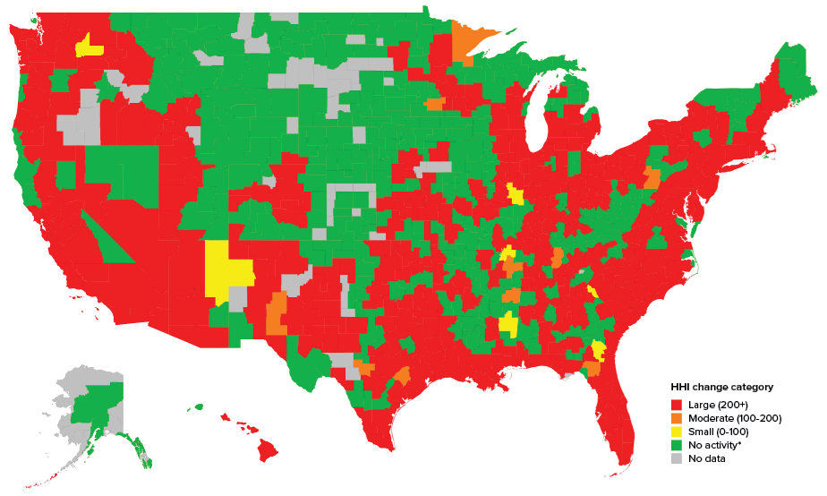
*Commuting zones without both active Sprint and T-Mobile stores
Note: The map shows, for each commuting zone, the change in the Herfindahl-Hirschman Index, a standard measure of market concentration, applied in this context to labor market concentration. A change of more than 200 HHI would trigger enforcement concerns per the Justice Department/Federal Trade Commission Horizontal Merger Guidelines.
Source: Change to Win 2018
Predicted concentration in the retail wireless labor market if Sprint and T-Mobile merge, by commuting zone
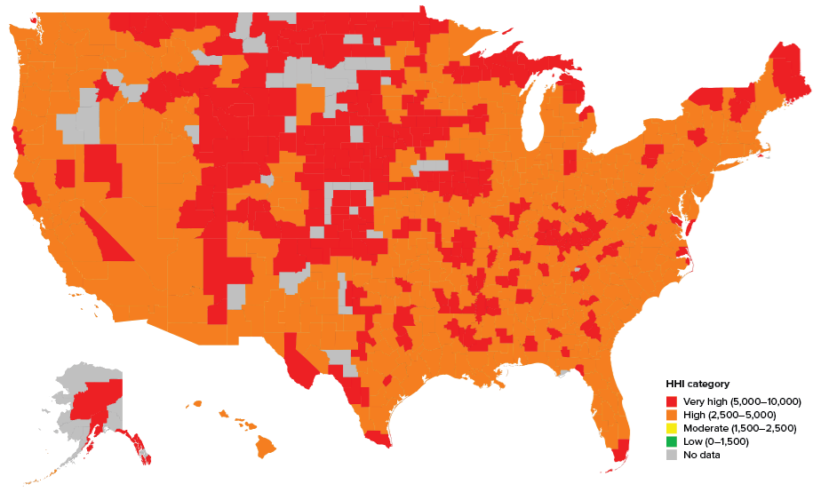
Note: The map shows, for each commuting zone, the predicted value of the Herfindahl-Hirschman Index, a standard measure of market concentration, applied in this context to labor market concentration. An HHI of 2,500 or more is considered “highly concentrated” under the Justice Department/Federal Trade Commission Horizontal Merger Guidelines.
Source: Change to Win 2018
The studies we rely on all estimate earnings-concentration regression equations of the form
![]()
where wit is the observed earnings in market i at time t, HHIit is market-level concentration, Xit are market-level time-varying controls, αi is a market-level fixed effect, γt represents time trends, and εit is the residual.7 The controls used in those studies differ depending on the data set: labor market tightness, for example, in the case of Azar, Marinescu, and Steinbaum 2017, is a way of controlling for the state of the within-market business cycle assumed to be caused by demand shocks.8
The analysis we conduct here is to ask how earnings would change given a change in concentration due to the merger, holding everything else constant.9 For that reason, we take the difference between two versions of the equation above, one for pre-merger and one for post-merger. That leaves us with
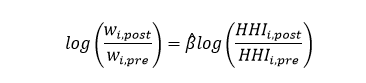
The ratio of HHIs is taken from the Change to Win 2018 estimates and the βs come from the three studies. We use them to return the log earnings ratio. We then exponentiate that to ascertain the percent change in earnings due to the counterfactual increase in concentration.
Specifically, we use a total of four estimates of β. From Azar, Marinescu, and Steinbaum 2017, we take specifications (3) and (6) from Table 2, Panel A. These include labor market tightness as well as fixed effects for commuting zones by occupations and commuting zones by quarter. Column (3) is an ordinary least squares (OLS) specification, and column (6) uses the instrumental variable from national changes in market-level firm counts. From Benmelech, Bergman, and Kim 2018, we use Table II, Panel B, column (6), which has both industry and year fixed effects, as well as labor productivity and other firm-level observables. From Rinz 2018, we use the specification in Table 7, column (4), which is similar to the instrumental variables one in Azar, Marinescu, and Steinbaum 2017, except that there is no tightness observable and the Rinz 2018 instrument uses concentration in other labor markets rather than the inverse of firm count in other labor markets. In each of these cases, the specification selected (see Table 2) is the one that (in our view) most closely matches the market definition used in the Change to Win 2018 concentration data.
Earnings elasticity by specification
| Study | Earnings elasticity (coefficient) |
|---|---|
| Azar et al. (OLS) | -0.0378 |
| Azar et al. (IV) | -0.127 |
| Benmelech et al. | -0.054* |
| Rinz | -0.0324 |
* Benmelech et al. is a “log-linear” specification, meaning that its magnitude is not comparable to the log–log specification of the other three coefficients.
Sources: Azar, Marinescu, and Steinbaum 2017 (“Azar et al.”); Benmelech, Bergman, and Kim 2018 (“Benmelech et al.”); Rinz 2018
The histograms in Figure E illustrate the predicted worker-earnings effect of the proposed Sprint–T-Mobile merger in each of the four specifications we use. In commuting zones where no change in concentration takes place (because either one or both of the merging parties isn’t present), there is no change in earnings. The variation among the four specifications that arises in these figures is due to the different estimates of β. In the highest-magnitude specification, Azar, Marinescu, and Steinbaum (2017) IV, the percent change in earning is as large as 7 percent in the labor market with the largest change in concentration. In most labor markets affected by the merger, the change in earnings is between 1 and 3 percent.
Predicted percent change in worker earnings due to the increase in retail wireless labor market concentration if Sprint and T-Mobile merge
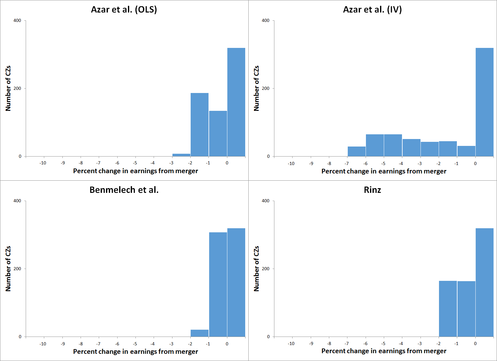
Note: “CZs” on y-axis stands for commuting zones. X-axis data labels indicate the lower bound of each bin. The right-most bar on each histogram represents the labor markets that are unaffected by the merger.
Source: Authors’ calculations based on data from Change to Win 2018. Individual panels show change in worker earnings using estimated effects of labor market concentration from Azar, Marinescu, and Steinbaum 2017 (“Azar et al.”); Benmelech, Bergman, and Kim 2018 (“Benmelech et al.”); and Rinz 2018 (see text for details).
In order to calculate dollar values of these earnings reductions, we apply the pre-/post-merger earnings ratios to actual earnings data from the Quarterly Census of Employment and Wages (QCEW) for NAICS Industry 443142. For that level of aggregation, the QCEW reports earnings data at the county level where there are sufficient observations to clear anonymity concerns. From there, we aggregate to commuting zones. For commuting zones with no earnings data from its constituent counties, we use the state-level earnings for that industry.
Given baseline QCEW earnings, we calculate the dollar value of the percent change in average earnings by commuting zone in each of the four specifications. Those are displayed in Figure F as scatterplots and in Figures G and H as commuting-zone-level color-coded maps.
Predicted change in retail wireless labor market concentration and in workers' weekly dollar earnings if Sprint and T-Mobile merge
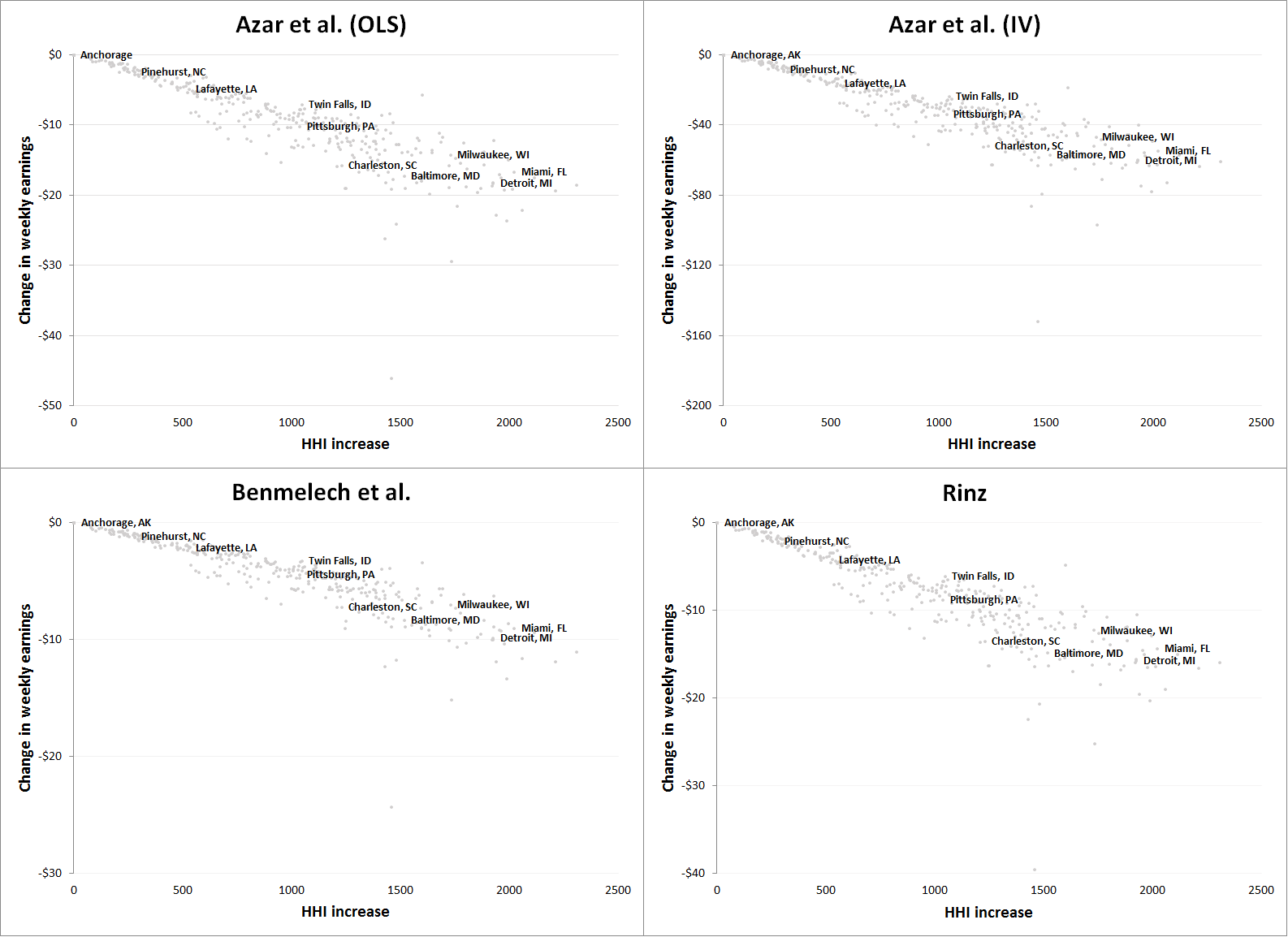
Note: Y-axis scales are different for each scatterplot. The x-axis shows the increase in the Herfindahl-Hirschman Index, a standard measure of market concentration, applied in this context to labor market concentration.
Source: Authors’ calculations based on data from Change to Win 2018 and earnings data from the Quarterly Census of Employment and Wages. Individual panels show change in labor market concentration and worker earnings using estimated effects of labor market concentration from Azar, Marinescu, and Steinbaum 2017 (“Azar et al.”); Benmelech, Bergman, and Kim 2018 (“Benmelech et al.”); and Rinz 2018. See text for details.
Predicted change in workers' weekly dollar earnings if Sprint and T-Mobile merge, by commuting zone (Azar et al. specifications)
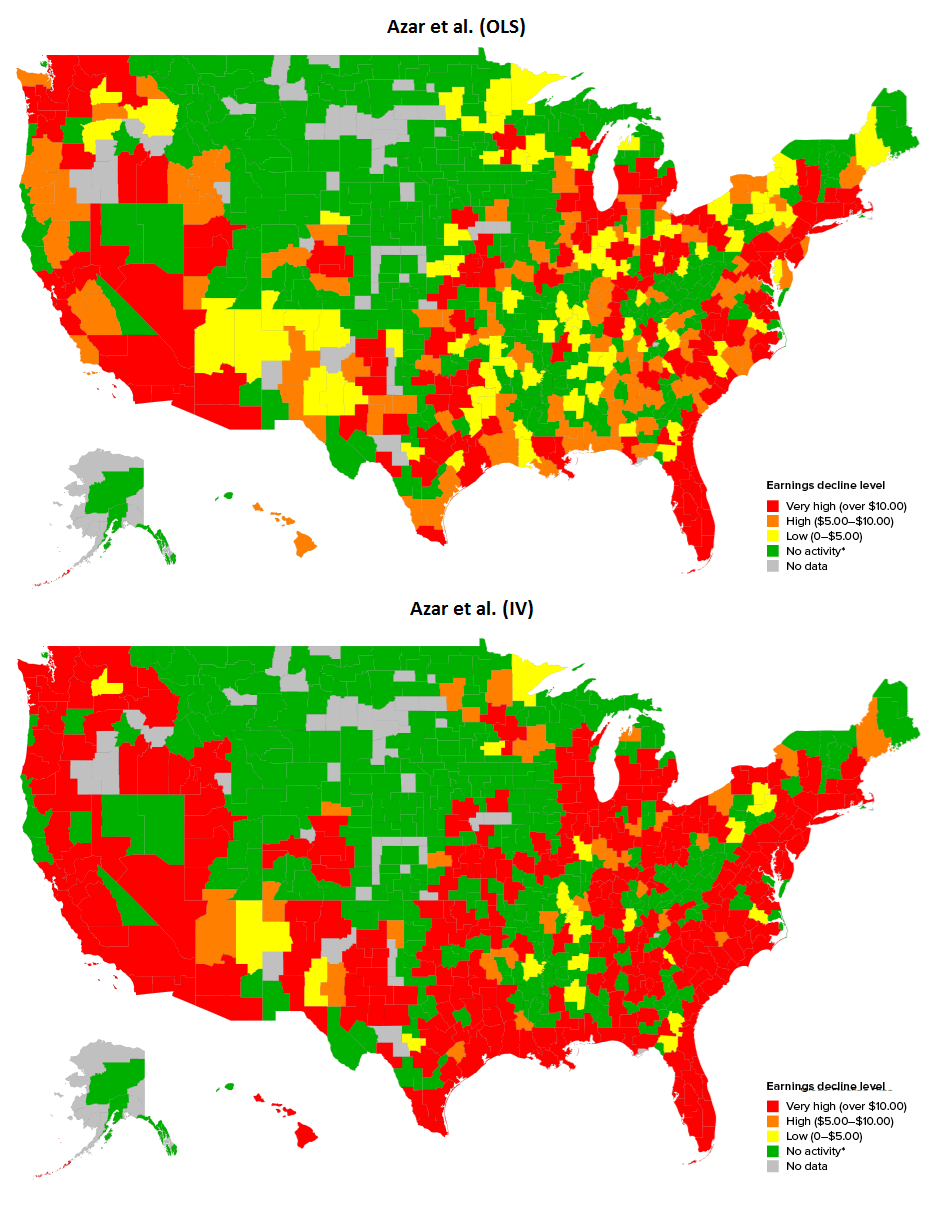
* Commuting zones without both active Sprint and T-Mobile stores
Source: Authors’ calculations based on data from Change to Win 2018 and earnings data from the Quarterly Census of Employment and Wages. Individual panels show change in labor market concentration and worker earnings using estimated effects of labor market concentration from Azar, Marinescu, and Steinbaum 2017 (“Azar et al.”). See text for details.
Predicted change in workers' weekly dollar earnings if Sprint and T-Mobile merge, by commuting zone (Benmelech et al. and Rinz specifications)
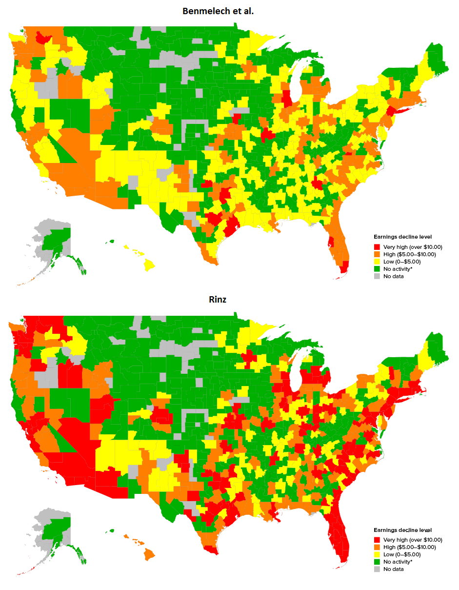
* Commuting zones without both active Sprint and T-Mobile stores
Source: Authors’ calculations based on data from Change to Win 2018 and earnings data from the Quarterly Census of Employment and Wages. Individual panels show change in labor market concentration and worker earnings using estimated effects of labor market concentration from Benmelech, Bergman, and Kim 2018 (“Benmelech et al.”); and Rinz 2018. See text for details.
Finally, we report the top 10 commuting zones ranked by the dollar value of the predicted earnings reductions for workers (shown in Table 3). The 10 most affected commuting zones in terms of weekly worker-earnings declines are identical across specifications, but the magnitude of the reduction differs. We report this to illustrate the extent of the harm to labor market competition done by the merger at its most severe. (See Appendix Tables 1 and 2 for the top 50 most affected commuting zones ranked by population and by the dollar value of the earnings decline.)
10 commuting zones with the largest predicted decline in retail wireless worker weekly earnings from a Sprint–T-Mobile merger
| Rank | Commuting zone | Azar et al. (OLS) | Azar et al. (IV) | Benmelech et al. | Rinz |
|---|---|---|---|---|---|
| 1 | Wenatchee, WA | -$46.03 | -$151.95 | -$24.33 | -$39.49 |
| 2 | Atlanta, GA | -$29.38 | -$96.63 | -$15.13 | -$25.22 |
| 3 | Newark, NJ | -$26.11 | -$86.05 | -$12.32 | -$22.40 |
| 4 | Philadelphia, PA | -$24.01 | -$79.14 | -$11.74 | -$20.61 |
| 5 | Dallas, TX | -$23.64 | -$77.65 | -$13.31 | -$20.29 |
| 6 | Chicago, IL | -$22.77 | -$74.71 | -$11.89 | -$19.54 |
| 7 | Witchita Falls, TX | -$22.14 | -$72.56 | -$11.58 | -$19.01 |
| 8 | St. Louis, MO | -$21.50 | -$70.61 | -$10.64 | -$18.45 |
| 9 | Washington, DC | -$19.73 | -$64.90 | -$9.63 | -$16.93 |
| 10 | Kansas City, KS | -$19.55 | -$64.14 | -$9.76 | -$16.78 |
Source: Authors’ calculations based on data from Change to Win 2018 and earnings data from the Quarterly Census of Employment and Wages. Data columns show change in labor market concentration and worker earnings using estimated effects of labor market concentration from Azar, Marinescu, and Steinbaum 2017 (“Azar et al.”); Benmelech, Bergman, and Kim 2018 (“Benmelech et al.”); and Rinz 2018. See text for details.
Discussion
This counterfactual analysis of merger effects potentially suffers from the methodological flaw that it may be economically incoherent to treat market concentration as an independent variable, even if estimates of its effect on earnings using the three studies are successful in uncovering exogenous variation in concentration in the data sets examined. This concern would vitiate the ceteris paribus exercise on which these predictions rest: that one can take before-and-after earnings-concentration equations and vary concentration without affecting other elements of market structure that might also affect the wage. The reason why is that concentration may be (and probably is) co-determined with other causes of earnings, or any equilibrium observable. For example, the Azar, Marinescu, and Steinbaum 2017 specifications control for labor market tightness in order to filter out demand shocks to local labor markets that might put some firms out of business, thus increasing concentration, and also lower earnings. Benmelech, Bergman, and Kim (2018) control for plant-level productivity to take into account that employers that are more productive are likely to have both higher market share and pay higher wages. In both cases, the change in concentration would be an effect, rather than a cause, of the same factor that changed wages. The exercise here assumes that you can vary concentration in these markets while leaving tightness or firm productivity unaffected, which may or may not be true in reality, even if the earnings regressions were able to filter out the effect of local labor demand shocks or of productivity.
While we recognize that these studies are not the last word on the effect of labor market concentration on workers’ earnings, there are good reasons to believe in their empirical relevance to this merger review. Most importantly, they are able to survive the usual endogeneity critiques of concentration regressions: that concentration is caused by firm-specific productivity that also causes whatever outcome is being investigated, or that some set of shocks (for example, to labor demand) causes both variation in concentration and variation in earnings. As the previous paragraph implies, however, the critique is not simply that the regressions in the studies are endogenous, but also that it is economically incoherent to vary concentration out of sample and consider the effect of doing so on outcomes. Our response to this is simply that taking such a critique to its logical conclusion would make it difficult to perform any economic-policy-relevant counterfactual. Economists recognize that independent variables are co-determined all the time and nonetheless perform counterfactuals on them, hopefully using empirical estimates that most closely mirror the counterfactual exercise being undertaken in an experimental or quasi-experimental setup.
The typical approach to merger review in product markets is to weigh the increased prices due to increased market power deriving from a merger-induced change to market structure against merger “efficiencies” resulting from reductions in suppliers’ costs. Since we are concerned exactly with such “efficiencies”—namely, the exercise of anti-competitive monopsony power in labor markets—we eschew the latter consideration, for which there is in any case no obvious counterpart on the seller side of the wireless telecommunications market, and because, as the aforementioned paper by Glick (2018) points out, the “tradeoff” is incoherent in welfare terms in any case. What distinguishes our assessment of earnings reductions from the analysis typically employed by antitrust agencies and courts is our direct analysis of the market in which market power is (potentially) being exercised, versus, for example, making assumptions about the form of competition in that market and deriving a mathematical model from those assumptions, within which the merger can then be simulated—conditional on the correctness of those assumptions. Whether one is willing to make those assumptions depends on what is to be gained from them. Here, we would rather not commit ourselves to specifying ex ante how competition in labor markets works. We prefer simply to go to the data.
A further source of concern about the accuracy of our predictions is that if we have defined labor markets incorrectly, then there may be greater elasticity of labor supply in response to increased market concentration (as we measure it) than there was in the samples of markets used by the studies we rely on. Intuitively, if our market definition is narrow relative to those studies, then workers may move more easily to other employers should the merging parties or their competitors seek to reduce wages. Perhaps retail employees in mobile telecoms stores can easily find work in other types of stores, for example.
This concern should be mitigated, however, by the studies of low firm-specific labor supply elasticity cited above (Webber 2015; Dube et al. 2018). What they find is that even where workers could easily find another job—for example, in online labor markets where work is interchangeable and any job can be done from the same place—namely, one’s home—the elasticity of labor supply with respect to the wage is extremely low. What appears to outside observers as abundant job opportunities available to workers seems not to be the case for the workers themselves. Strengthening the case that a narrow market definition is appropriate is the fact that Sprint and T-Mobile have been known to use noncompete agreements to constrain the mobility of their workers (PerfectHandle 2015; Nevs0521 2006).
Finally, a more mundane objection to this exercise, but one worth making since it is more grounded in the empirics of prospective and retrospective merger analysis, is that concentration is highly variable even in well-defined antitrust markets, for reasons other than mergers. Ex-post examination of competitive effects of a merger often have trouble even detecting any merger effect on concentration outside of the most-affected markets, let alone the competitive effect of that change in concentration on outcomes (Steinbaum 2018). That is because the merger “signal” is often drowned out by the noise of other variation in concentration, from entry, exit, or changes in market shares arising from some other cause. In this paper’s exercise, the variation in concentration we use to predict earnings changes is calculated by simply combining market shares of the merging parties. But should the merger be consummated, the change in concentration that actually results from it would probably be different (and vary widely across markets) than the predicted change we use. That concern is prior to the concern about the out-of-sample robustness of the earnings regressions, and probably a more empirically relevant basis for doubting these predictions than the reluctance to make assumptions about the competitive structure of labor markets expressed above.
Conclusion and policy implications
In this paper, we predict that the merger of Sprint and T-Mobile would reduce labor market competition and therefore reduce earnings in the labor markets where the combined company hires workers to staff its retail stores. To do that, we employ earnings-concentration estimates from three recent studies, which use distinct data sets and specifications to estimate a negative relationship. Moreover, there is reason to believe this market, like most labor markets, is already monopsonized, and hence a profit-maximizing employer would be expected to use its increased monopsony power to reduce wages and worker benefits post-merger.
To the best of our knowledge, this is the first attempt to use the recent spate of labor market concentration studies in a prospective merger review in the United States. We think that analysis of competitive effects in labor markets should be incorporated into competition enforcement as a routine matter. This would require antitrust agencies to come up with principles for defining labor markets and assessing competition therein. It would also involve compulsory data collection from merging parties and other market participants with respect to firm- and establishment-level payroll data matched to employee characteristics (including labor market histories), insofar as these are known to the firms. It should encompass restrictions employers place on their workers, including noncompetes and mandatory arbitration clauses and class-action waivers. It should also extend to independent contractors and other non-employee workers, given their increasing importance to the business models of the economy’s most powerful actors. Given what we know about the high degree of interfirm and interestablishment disparities in pay, and what the research shows about the importance of internal labor markets, promotion structures, hiring policies, and outsourcing for labor market outcomes, highly granular data is necessary to effectively assess competition implications for labor markets. Furthermore, if such data collection were a routine (and compulsory) part of merger review, then we would not need to rely on out-of-sample predictions of earnings effects such as the one undertaken in this paper; instead, we could look at wage and other labor data connected directly to the merging parties, as employers.
The potential for anti-competitive effects of mergers in labor markets implicates larger issues of antitrust enforcement beyond expanding merger review to consider labor markets. Under the consumer welfare standard, when evaluating the potential for the anti-competitive exercise of monopoly power, enforcers weigh harm to consumers against “efficiencies” in the form of lower costs of production. If monopsony power is endemic in the economy, then such a comparison is incoherent in welfare economics terms because the profits of incumbents due to anti-competitive wage reductions are not equivalent in welfare terms to consumer surplus. This scenario points to the inadequacy of the consumer welfare standard to antitrust enforcement given realistic economic assumptions.
For that reason, we have proposed the Effective Competition Standard (Steinbaum and Stucke 2018), which, if enacted, would alter the Sprint–T-Mobile merger review in three respects. First of all, it shifts the burden of proof in any merger review to the merging parties, to prove their transaction would not harm competition. Second, it mandates that antitrust enforcers look more often upstream for anti-competitive effects, including in labor markets—mitigating the neglect of upstream harm to competition during the consumer welfare standard era. Finally, it establishes a right of market access for upstream suppliers, which, in this case, would include content creators who use wireless technology to reach customers. They would have the right to do so without exclusion or discrimination, which in turn places restrictions on the autonomy of powerful telecoms distributors like a combined Sprint–T-Mobile to extract a toll or to treat their customers or affiliates preferentially. If the merger threatened that right of market access, that would be grounds for preventing it.
This merger is proposed in a market where product market competition has been virtually eliminated, by both horizontal and vertical mergers and through the repeal of regulations—the 2015 Open Internet Order—designed to preserve competition in a sector in which incentives for discrimination and exclusion are significant. The aim of the Telecommunications Act of 1996—to introduce competition as an alternative to the heavy-handed regulation of the regime established by the Communications Act of 1934 and amendments—has manifestly failed. Instead, we now have the worst of both worlds: private rather than public regulation; discrimination and exclusion among suppliers, workers, and customers; and the extremely high profits that result from such a business model. Moreover, the labor markets where telecoms companies hire their workers are already monopsonized, meaning that increased market power on the part of employers would likely cause employment loss and wage declines. It is time for competition and regulatory authorities to take a new look at the rules governing the way telecoms are currently run in this country, including the antitrust enforcement approach that has allowed telecoms companies to consolidate to the point that they threaten overall economic well-being.
Acknowledgments
The authors, the Economic Policy Institute, and the Roosevelt Institute thank the Communications Workers of America for its support for this project. The report reflects the views of the authors but was reviewed by the CWA prior to publication.
About the authors
Adil Abdela is a Research Associate at the Roosevelt Institute.
Marshall Steinbaum is Research Director and a Fellow at the Roosevelt Institute.
Appendix
Predicted decline in retail wireless worker weekly earnings from a Sprint–T-Mobile merger, by commuting zone, ranked by population size
| Rank (by population) | Commuting zone | Azar et al. (OLS) | Azar et al. (IV) | Benmelech et al. | Rinz |
|---|---|---|---|---|---|
| 1 | Los Angeles, CA | -$16.96 | -$55.69 | -$9.14 | -$14.56 |
| 2 | New York, NY | -$18.91 | -$62.24 | -$10.07 | -$16.23 |
| 3 | Chicago, IL | -$22.77 | -$74.71 | -$11.89 | -$19.54 |
| 4 | Houston, TX | -$18.58 | -$61.03 | -$10.03 | -$15.95 |
| 5 | Newark, NJ | -$24.01 | -$79.14 | -$11.74 | -$20.61 |
| 6 | San Francisco, CA | -$17.16 | -$56.59 | -$8.10 | -$14.73 |
| 7 | Boston, MA | -$11.82 | -$39.05 | -$5.55 | -$10.14 |
| 8 | Washington, DC | -$19.73 | -$64.90 | -$9.63 | -$16.93 |
| 9 | Atlanta, GA | -$29.38 | -$96.63 | -$15.13 | -$25.22 |
| 10 | Philadelphia, PA | -$12.37 | -$40.88 | -$5.80 | -$10.61 |
| 11 | Detroit, MI | -$18.29 | -$60.07 | -$9.83 | -$15.70 |
| 12 | Miami, FL | -$19.33 | -$63.47 | -$11.86 | -$16.59 |
| 13 | Phoenix, AZ | -$15.45 | -$50.97 | -$7.69 | -$13.26 |
| 14 | Seattle, WA | -$18.98 | -$62.71 | -$9.05 | -$16.28 |
| 15 | Dallas, TX | -$23.64 | -$77.65 | -$13.31 | -$20.29 |
| 16 | New Haven, CT | -$11.91 | -$39.40 | -$5.22 | -$10.22 |
| 17 | Minneapolis, MN | -$18.15 | -$59.81 | -$8.48 | -$15.58 |
| 18 | San Diego, CA | -$13.74 | -$45.27 | -$6.92 | -$11.79 |
| 19 | Tampa, FL | -$18.73 | -$61.62 | -$10.29 | -$16.07 |
| 20 | Denver, CO | -$13.27 | -$43.67 | -$6.42 | -$11.39 |
| 21 | Baltimore, MD | -$17.26 | -$56.86 | -$8.34 | -$14.82 |
| 22 | Akron, OH | -$12.30 | -$40.54 | -$5.67 | -$10.55 |
| 23 | San Jose, CA | -$15.82 | -$52.26 | -$7.25 | -$13.57 |
| 24 | St. Louis, MO | -$21.50 | -$70.61 | -$10.64 | -$18.45 |
| 25 | Pittsburgh, PA | -$10.24 | -$33.88 | -$4.47 | -$8.78 |
| 26 | Yonkers, NY | -$11.78 | -$38.95 | -$5.49 | -$10.11 |
| 27 | Sacremento, CA | -$13.48 | -$44.44 | -$6.43 | -$11.57 |
| 28 | Orlando, FL | -$17.51 | -$57.45 | -$9.26 | -$15.03 |
| 29 | Portland, Oregon | -$12.12 | -$40.00 | -$5.60 | -$10.40 |
| 30 | Lake Havasu, AZ | -$12.66 | -$41.75 | -$5.98 | -$10.86 |
| 31 | Dallas, TX | -$18.15 | -$59.65 | -$9.97 | -$15.58 |
| 32 | San Antonio, TX | -$17.04 | -$56.08 | -$8.66 | -$14.63 |
| 33 | Cincinnati, OH | -$13.86 | -$45.69 | -$6.24 | -$11.89 |
| 34 | Charolotte, NC | -$13.52 | -$44.53 | -$6.16 | -$11.60 |
| 35 | Columbus, OH | -$17.66 | -$58.16 | -$8.21 | -$15.16 |
| 36 | Indianapolis, IN | -$15.07 | -$49.69 | -$6.88 | -$12.94 |
| 37 | Durham, NC | -$16.72 | -$55.16 | -$7.67 | -$14.35 |
| 38 | Kansas City, KS | -$19.55 | -$64.14 | -$9.76 | -$16.78 |
| 39 | Atlantic City, NJ | -$16.46 | -$54.28 | -$7.85 | -$14.12 |
| 40 | Austin, TX | -$26.11 | -$86.05 | -$12.32 | -$22.40 |
| 41 | Fort Lauderdale, FL | -$16.72 | -$54.84 | -$9.01 | -$14.35 |
| 42 | York, PA | -$10.62 | -$35.07 | -$4.77 | -$9.11 |
| 43 | Milwaukee, WI | -$14.26 | -$46.85 | -$7.01 | -$12.24 |
| 44 | Virginia Beach, VA | -$11.06 | -$36.46 | -$5.24 | -$9.49 |
| 45 | Salt Lake City, UT | -$16.69 | -$55.02 | -$8.05 | -$14.32 |
| 46 | Hanford, CA | -$9.08 | -$30.03 | -$4.12 | -$7.79 |
| 47 | Providence, RI | -$14.66 | -$48.16 | -$7.32 | -$12.58 |
| 48 | Jacksonville, FL | -$17.30 | -$56.94 | -$8.65 | -$14.85 |
| 49 | Nashville, TN | -$16.36 | -$53.92 | -$7.38 | -$14.04 |
| 50 | Grand Rapids, MI | -$17.41 | -$57.36 | -$9.04 | -$14.94 |
Source: Authors’ calculations based on data from Change to Win 2018 and earnings data from the Quarterly Census of Employment and Wages. Data columns show change in labor market concentration and worker earnings using estimated effects of labor market concentration from Azar, Marinescu, and Steinbaum 2017 (“Azar et al.”); Benmelech, Bergman, and Kim 2018 (“Benmelech et al.”); and Rinz 2018. See text for details.
Predicted decline in retail wireless worker weekly earnings from a Sprint–T-Mobile merger, by commuting zone, ranked by earnings change
| Rank (by earnings change) | Commuting zone | Azar et al. (OLS) | Azar et al. (IV) | Benmelech et al. | Rinz |
|---|---|---|---|---|---|
| 1 | Wenatchee, WA | -$46.03 | -$151.95 | -$24.33 | -$39.49 |
| 2 | Atlanta, GA | -$29.38 | -$96.63 | -$15.13 | -$25.22 |
| 3 | Austin, TX | -$26.11 | -$86.05 | -$12.32 | -$22.40 |
| 4 | Newark, NJ | -$24.01 | -$79.14 | -$11.74 | -$20.61 |
| 5 | Dallas, TX | -$23.64 | -$77.65 | -$13.31 | -$20.29 |
| 6 | Chicago, IL | -$22.77 | -$74.71 | -$11.89 | -$19.54 |
| 7 | Wichita Falls, TX | -$22.14 | -$72.56 | -$11.58 | -$19.01 |
| 8 | St. Louis, MO | -$21.50 | -$70.61 | -$10.64 | -$18.45 |
| 9 | Washington, DC | -$19.73 | -$64.90 | -$9.63 | -$16.93 |
| 10 | Kansas City, KS | -$19.55 | -$64.14 | -$9.76 | -$16.78 |
| 11 | Miami, FL | -$19.33 | -$63.47 | -$11.86 | -$16.59 |
| 12 | Martinsville, VA | -$19.22 | -$63.09 | -$10.35 | -$16.50 |
| 13 | El Centro, CA | -$19.10 | -$62.61 | -$9.93 | -$16.40 |
| 14 | Provo-Orem, UT | -$19.05 | -$62.75 | -$8.86 | -$16.35 |
| 15 | Columbia, SC | -$19.03 | -$62.64 | -$8.90 | -$16.34 |
| 16 | Champaign, IL | -$18.98 | -$62.65 | -$8.41 | -$16.29 |
| 17 | Seattle, WA | -$18.98 | -$62.71 | -$9.05 | -$16.28 |
| 18 | New Orlean, LA | -$18.98 | -$62.26 | -$9.49 | -$16.29 |
| 19 | New York, NY | -$18.91 | -$62.24 | -$10.07 | -$16.23 |
| 20 | Tampa, FL | -$18.73 | -$61.62 | -$10.29 | -$16.07 |
| 21 | Houston, TX | -$18.58 | -$61.03 | -$10.03 | -$15.95 |
| 22 | St. Joseph, MO | -$18.53 | -$60.76 | -$11.05 | -$15.91 |
| 23 | Detroit, MI | -$18.29 | -$60.07 | -$9.83 | -$15.70 |
| 24 | Boise City, ID | -$18.17 | -$59.77 | -$8.54 | -$15.60 |
| 25 | Dallas, TX | -$18.15 | -$59.65 | -$9.97 | -$15.58 |
| 26 | Minneapolis, MN | -$18.15 | -$59.81 | -$8.48 | -$15.58 |
| 27 | Huntsville, TX | -$17.89 | -$58.91 | -$8.98 | -$15.35 |
| 28 | Columbus, OH | -$17.66 | -$58.16 | -$8.21 | -$15.16 |
| 29 | Orlando, FL | -$17.51 | -$57.45 | -$9.26 | -$15.03 |
| 30 | Plainview, TX | -$17.45 | -$57.47 | -$9.17 | -$14.97 |
| 31 | Ottawa, KS | -$17.43 | -$57.10 | -$9.36 | -$14.96 |
| 32 | Grand Rapids, MI | -$17.41 | -$57.36 | -$9.04 | -$14.94 |
| 33 | Jacksonville, FL | -$17.30 | -$56.94 | -$8.65 | -$14.85 |
| 34 | Greenville, NC | -$17.29 | -$56.91 | -$9.18 | -$14.84 |
| 35 | Baltimore, MD | -$17.26 | -$56.86 | -$8.34 | -$14.82 |
| 36 | San Francisco, CA | -$17.16 | -$56.59 | -$8.10 | -$14.73 |
| 37 | San Antonio, TX | -$17.04 | -$56.08 | -$8.66 | -$14.63 |
| 38 | Los Angeles, CA | -$16.96 | -$55.69 | -$9.14 | -$14.56 |
| 39 | Durham, NC | -$16.72 | -$55.16 | -$7.67 | -$14.35 |
| 40 | Fort Lauderdale, FL | -$16.72 | -$54.84 | -$9.01 | -$14.35 |
| 41 | Salt Lake City, UT | -$16.69 | -$55.02 | -$8.05 | -$14.32 |
| 42 | Atlantic City, NJ | -$16.46 | -$54.28 | -$7.85 | -$14.12 |
| 43 | Nashville, TN | -$16.36 | -$53.92 | -$7.38 | -$14.04 |
| 44 | Flint, MI | -$16.21 | -$53.25 | -$8.16 | -$13.92 |
| 45 | San Jose, CA | -$15.82 | -$52.26 | -$7.25 | -$13.57 |
| 46 | Harrisonburg, VA | -$15.78 | -$52.00 | -$9.02 | -$13.54 |
| 47 | Charleston, SC | -$15.72 | -$51.91 | -$7.22 | -$13.49 |
| 48 | Emporia, KS | -$15.65 | -$51.42 | -$8.33 | -$13.43 |
| 49 | Phoenix, AZ | -$15.45 | -$50.97 | -$7.69 | -$13.26 |
| 50 | Ontario, OR | -$15.43 | -$50.70 | -$7.69 | -$13.25 |
| Average | -$19.13 | -$62.93 | -$9.74 | -$16.42 |
* Rankings are based on the Azar et al. (OLS) predicted earnings decline.
Source: Authors’ calculations based on data from Change to Win 2018 and earnings data from the Quarterly Census of Employment and Wages. Data columns show change in labor market concentration and worker earnings using estimated effects of labor market concentration from Azar, Marinescu, and Steinbaum 2017 (“Azar et al.”); Benmelech, Bergman, and Kim 2018 (“Benmelech et al.”); and Rinz 2018. See text for details.
Endnotes
1. The new findings we put to use in this paper on monopsony power in labor markets return to the roots of an old debate about whether individual employers have the power to set wages (which is how this paper defines “monopsony”). In recent decades, economists have grounded their theories as to why individual employers have the power to set wages in labor market imperfections that impair worker mobility even when many employers might be active in a given market (Manning 2003, 2011). The three papers we rely on for the predictions made in this paper resurrect arguments in an older literature—that employer power to set wages might also be caused by outright concentration, i.e., the existence of few employers in a given labor market, which means that workers cannot obtain outside job offers because there aren’t any employers to give job offers (Robinson 1933, for example). We view the two theories as consistent and mutually reinforcing, with implications for competition policy that are considerable.
2. The Herfindahl-Hirschman Index is computed by summing the squares of each firm’s market share, and then multiplying the resulting sum by 10,000. It thus up-weights large market shares in the computation of overall concentration in a market.
3. According to the Horizontal Merger Guidelines, the threshold for a highly concentrated market is 2500, and the threshold for a merger that threatens to reduce competition is one that would increase concentration by 200 HHI points.
4. 374 U.S. 321.
5. The word “monopsony” formally refers to a single employer as the sole purchaser of labor in a market, but the word has a wider application in this paper and in the economics literature more generally. In contemporary economics, monopsony power refers to inelastic firm-level labor supply, giving employers some unilateral discretion to set wages. Alternatively, from the worker’s point of view, monopsony refers to wages that are less than the marginal product of labor. There are many potential reasons why labor markets might be monopsonized, including a small number of employers, search-and-matching frictions, asymmetric information, or discrimination.
6. Change to Win’s research indicates that the Sprint–T-Mobile merger is likely to reduce employment by the merging parties and their competitors. The analysis in this EPI paper assumes no change in employment as a result of the merger. The analysis in this paper could be seen, for that reason, as a scenario under which the monopsony power that results from the merger is used solely to depress wages. In reality, it may reduce both wages and employment.
7. Benmelech, Bergman, and Kim (2018) use a log-level, rather than a log–log, specification for the earnings-concentration regression equation. This difference is reflected in the merger counterfactual calculations reported below.
8. Benmelech, Bergman, and Kim (2018) observe unionization rates at firms in their data, which they use as another control. They find that unionization mitigates the earnings-reducing effect of concentration, a finding that is tentatively corroborated by Kwan and Liu (2018). In fact, the Benmelech, Bergman, and Kim 2018 paper posits that one of the reasons labor market concentration exerts a macroeconomically significant negative impact on wages now, versus in the past, is not only that labor markets have become more concentrated, but also that concentration matters more for wages since unionization rates have declined. For the retail wireless labor markets we study, Change to Win (2018) estimates that the unionization rate is approximately 9 percent, almost entirely at corporately owned stores of AT&T Mobility LLC (the AT&T subsidiary that provides wireless services).
9. We return to the validity of this ceteris paribus exercise for concentration at the end of this section.
References
Azar, José, Ioana Marinescu, and Marshall Steinbaum. 2017. “Labor Market Concentration.” National Bureau of Economic Research Working Paper no. 24147, December 2017.
Azar, José, Ioana Marinescu, Marshall Steinbaum, and Bledi Taska. 2018. “Concentration in US Labor Markets: Evidence from Online Vacancy Data.” National Bureau of Economic Research Working Paper no. 24395, last updated August 2018.
Bartik, Alexander. 2018. “Moving Costs and Worker Adjustment to Changes in Labor Demand: Evidence from Longitudinal Census Data.” Working paper, October 2018.
Benmelech, Efraim, Nittai Bergman, and Hyunseob Kim. 2018. “Strong Employers and Weak Employees: How Does Employer Concentration Affect Wages?” National Bureau of Economic Research Working Paper no. 24307, February 2018.
Bloom, Nicholas, Fatih Guvenen, Benjamin S. Smith, Jae Song, and Till von Wachter. 2018. “Inequality and the Disappearing Large Firm Wage Premium.” AEA Papers and Proceedings 108 (May): 317–322.
Bureau of Labor Statistics (BLS). 2018. “All Employees, Thousands, Retail Trade, Seasonally Adjusted” [Excel file], Employment, Hours, and Earnings from the Current Employment Statistics Survey (National). Accessed December 2018.
Bureau of Labor Statistics, Current Employment Statistics (BLS-CES). Various years. Public data series accessed through the CES National Databases and through series reports. Accessed December 2018.
Bureau of Labor Statistics, Quarterly Census of Employment and Wages (BLS-QCEW). Various years. Public data series accessed through the QCEW Databases and through series reports. Accessed December 2018.
Cengiz, Doruk, Arindrajit Dube, Attila Lindner, and Ben Zipperer. 2018. “The Effect of Minimum Wages on Low-Wage Jobs: Evidence from the United States Using a Bunching Estimator.” Centre for Economic Performance Discussion Paper no. 1531, February 2018.
Change to Win. 2018. “2018 Wireless Retail Employment Estimates.” Unpublished Excel files provided by Change to Win, Washington, D.C.
Chaplin, Jonathan, Spencer Kurn, Vivek Stalam, and Robert Shuffield. 2018. Sprint / T-Mobile Redux: Refreshing Synergies and Scenarios. New Street Research, April 2018.
Cooper, David, Lawrence Mishel, and John Schmitt. 2015. We Can Afford a $12.00 Federal Minimum Wage in 2020. Economic Policy Institute Briefing Paper no. 398, April 2015.
Dube, Arindrajit, Laura Giuliano, and Jonathan Leonard. 2015. “Fairness and Frictions: Impact of Unequal Raises on Quit Behavior.” IZA Discussion Paper no. 9149.
Dube, Arindrajit, Jeff Jacobs, Suresh Naidu, and Siddharth Suri. 2018. “Monopsony in Online Labor Markets.” National Bureau of Economic Research Working Paper no. 24416.
Dube, Arindrajit, and Ethan Kaplan. 2010. “Does Outsourcing Reduce Wages in the Low-Wage Service Occupations? Evidence from Janitors and Guards.” ILR Review 63, no. 2 (January): 287–306.
Ganapati, Sharat. 2018. “Oligopolies, Prices, Output, and Productivity.” Working paper, last updated October 2018.
Glick, Mark. 2018. “The Unsound Theory Behind the Consumer (and Total) Welfare Standard in Antitrust.” Roosevelt Institute Working Paper, November 2018.
Goldman, Debbie, Allen Grunes, and Maurice E. Stucke. 2018. “Comments of Communications Workers of America Before the Federal Communications Commission, in the Matter of Applications of T-Mobile US, Inc., and Sprint Corporation for Consent to Transfer Control of the Licenses and Authorizations, WT Docket No. 18-197.” Public Comment, August 27, 2018.
Hemphill, C. Scott, and Nancy L. Rose. 2018. “Mergers That Harm Sellers.” Yale Law Journal 127, no. 7 (May): 2078–2109.
Hortaçsu, Ali, and Chad Syverson. 2015. “The Ongoing Evolution of US Retail: A Format Tug-of-War.” Journal of Economic Perspectives 29, no. 4 (Fall): 89–112. https://doi.org/10.1257/jep.29.4.89.
Hwang, Andrew, and Marshall I. Steinbaum. 2017. Crossed Lines: Why the AT&T-Time Warner Merger Demands a New Approach to Antitrust. Roosevelt Institute, February 2017.
Hyatt, Henry, and James Spletzer. 2016. “The Shifting Job Tenure Distribution.” Labour Economics 41, no. 1 (August): 363–377.
Konczal, Mike, and Marshall Steinbaum. 2016. Declining Entrepreneurship, Business Dynamism, and Labor Mobility: A Demand-Side Approach. Roosevelt Institute, July 2016.
Kwan, Alan, and Yukun Liu. 2018. “Labor Market Power and Firm Financial Flexibility.” Working paper, last updated April 2018. https://doi.org/10.2139/ssrn.3144130.
Manning, Alan. 2003. Monopsony in Motion: Imperfect Competition in Labor Markets. Princeton: Princeton Univ. Press.
Manning, Alan. 2011. “Imperfect Competition in the Labor Market.” In Handbook of Labor Economics, vol. 4, edited by Orley Ashenfelter and David Card, 973–1041. Elsevier.
Marinescu, Ioana, and Herbert J. Hovenkamp. 2018. “Anticompetitive Mergers in Labor Markets.” Faculty Scholarship no. 1965 (February 2018).
Molloy, Raven, Christopher L. Smith, Ricardo Trezzi, and Abigail Wozniak. 2016. “Understanding Declining Fluidity in the U.S. Labor Market.” Brookings Papers on Economic Activity 47, no. 1 (Spring): 183–259.
Naidu, Suresh, Eric A. Posner, and E. Glen Weyl. 2018. “Antitrust Remedies for Labor Market Power.” Harvard Law Review, forthcoming. https://doi.org/10.2139/ssrn.319221.
Nevs0521. 2006. “Non-Compete Clause?” (forum post). Howard Forums Mobile Community (online discussion board), October 4, 2006.
Ohlhausen, Maureen. 2017. “Letter to Senator Cory Booker.” December 1, 2017. Unpublished.
PerfectHandle. 2015. “Quick Question for the T-Mo Employees Here” (forum post). r/tmobile, reddit.com, February 26, 2015.
Rinz, Kevin. 2018. “Labor Market Concentration, Earnings Inequality, and Earnings Mobility.” CARRA Working Paper no. 2018–10.
Robinson, Joan. 1933. The Economics of Imperfect Competition. London: MacMillan.
Rossi-Hansberg, Esteban, Pierre-Daniel Sarte, and Nicholas Trachter. 2018. “Diverging Trends in National and Local Concentration.” National Bureau of Economic Research Working Paper no. 25066, September 2018.
Simons, Joseph. 2018. “Responses to Questions for the Record in re Testimony Before the United States Senate Committee on the Judiciary, Subcommittee on Antitrust, Competition Policy and Consumer Rights for a Hearing on ‘Oversight of the Enforcement of the Antitrust Laws,’ October 3, 2018.” Published November 6, 2018.
Song, Jae, David J. Price, Fatih Guvenen, Nicholas Bloom, and Till von Wachter. 2018. “Firming Up Inequality.” Quarterly Journal of Economics, forthcoming. https://doi.org/10.1093/qje/qjy025.
Steinbaum, Marshall. 2018. Airline Consolidation, Merger Retrospectives, and Oil Price Pass-Through. Roosevelt Institute, June 2018.
Steinbaum, Marshall, and Maurice E. Stucke. 2018. The Effective Competition Standard: A New Standard for Antitrust. Roosevelt Institute, September 2018.
Webber, Douglas A. 2015. “Firm Market Power and the Earnings Distribution.” Labour Economics 35 (August): 123–134. https://doi.org/10.1016/j.labeco.2015.05.003.
Weil, David. 2014. The Fissured Workplace: Why Work Became So Bad for So Many and What Can Be Done to Improve It. Cambridge, Mass.: Harvard Univ. Press.
Yagan, Danny. 2018. “Employment Hysteresis from the Great Recession.” Journal of Political Economy, forthcoming. Working paper (last updated August 2018), available at https://eml.berkeley.edu/~yagan/Hysteresis.pdf.
